用户购买CD行为数据分析
%matplotlib inline
# 正常显示中文
from pylab import matplotlib
matplotlib.rcParams['font.sans-serif'] = ['SimHei']
# 正常显示符号
matplotlib.rcParams['axes.unicode_minus']=False
import pandas as pd
import numpy as np
from matplotlib import pyplot as plt
# 读取数据
columns = ['user_id', 'order_dt', 'order_products', 'order_amount']
date = pd.read_table('CD.txt', names=columns, sep='\s+', engine='python')
print(date.head())# 将时间序列转化为时间格式
date['order_dt'] = pd.to_datetime(date['order_dt'], format='%Y%m%d')
# 转化为月份格式
date['month'] = date['order_dt'].values.astype('datetime64[M]')
   user_id  order_dt  order_products  order_amount
0        1  19970101               1         11.77
1        2  19970112               1         12.00
2        2  19970112               5         77.00
3        3  19970102               2         20.76
4        3  19970330               2         20.76
# 进行用户消费趋势的分析(按月)
group_month = date.groupby('month')
# 1. 每月的消费总金额
m_money = group_month['order_amount'].sum()
print(m_money.head())
plt.figure(figsize=(10,8), dpi=80)
plt.plot(m_money.index, m_money.values)
# m_money.plot()
plt.xticks(rotation=45)
plt.style.use('ggplot')
plt.show()
month
1997-01-01    299060.17
1997-02-01    379590.03
1997-03-01    393155.27
1997-04-01    142824.49
1997-05-01    107933.30
Name: order_amount, dtype: float64
![]()
从图中可以看出1997年前三个月销量比较高,随后一直到1998年消费下降并保持微小波动
# 2. 每月的消费次数
num_consume = group_month.count()['user_id']
print(num_consume.head())
plt.figure(figsize=(10,8), dpi=80)
plt.plot(num_consume.index, num_consume.values)
# m_money.plot()
plt.xticks(rotation=45)
plt.style.use('ggplot')
plt.show()
month
1997-01-01     8928
1997-02-01    11272
1997-03-01    11598
1997-04-01     3781
1997-05-01     2895
Name: user_id, dtype: int64
![]()
从上图可以看出,1997年前三个月有比较高的消费次数,三月达到最高,但随后一直到1998年消费次数下降并在一定范围内有些许波动
# 3. 每月的产品购买量
num_product = group_month['order_products'].sum()
print(num_product.head())
plt.figure(figsize=(10,8), dpi=80)
plt.plot(num_product.index, num_product.values)
# m_money.plot()
plt.xticks(rotation=45)
plt.style.use('ggplot')
plt.show()
month
1997-01-01    19416
1997-02-01    24921
1997-03-01    26159
1997-04-01     9729
1997-05-01     7275
Name: order_products, dtype: int64
![]()
# 4. 每月的消费人数
num_person = date.groupby(['month', 'user_id']).count()
num_person = num_person.reset_index('user_id').groupby('month').count()
print(num_person.head())
plt.figure(figsize=(10,8), dpi=80)
plt.plot(num_person.index, num_person.values)
# m_money.plot()
plt.xticks(rotation=45)
plt.style.use('ggplot')
plt.show()
            user_id  order_dt  order_products  order_amount
month
1997-01-01     7846      7846            7846          7846
1997-02-01     9633      9633            9633          9633
1997-03-01     9524      9524            9524          9524
1997-04-01     2822      2822            2822          2822
1997-05-01     2214      2214            2214          2214
![]()
每月消费人数低于每月消费次数,但差异不太大,前三个月每月的消费人数在8000-10000之间,随后平均消费人数为2000左右波动
date.pivot_table(index=['month'], values=['order_products', 'order_amount', 'user_id'],aggfunc={'order_products':'sum', 'order_amount':'sum', 'user_id':'count'}).head()
| order_amount | order_products | user_id | |
|---|---|---|---|
| month | |||
| 1997-01-01 | 299060.17 | 19416 | 8928 |
| 1997-02-01 | 379590.03 | 24921 | 11272 |
| 1997-03-01 | 393155.27 | 26159 | 11598 |
| 1997-04-01 | 142824.49 | 9729 | 3781 |
| 1997-05-01 | 107933.30 | 7275 | 2895 |
avg_consume = date.pivot_table(index=['month'], values=['order_amount'],aggfunc='mean')
# 5. 每月用户平均消费金额趋势
# count_consume = date.groupby('month')['order_amount'].count()
# all_consume = date.groupby('month')['order_amount'].sum()
# avg_consume = all_consume / count_consumeprint(avg_consume.head())
plt.figure(figsize=(10,8), dpi=80)
plt.plot(avg_consume.index, avg_consume.order_amount)
# m_money.plot()
plt.xticks(rotation=45)
plt.style.use('ggplot')
plt.show()
            order_amount
month
1997-01-01     33.496883
1997-02-01     33.675482
1997-03-01     33.898540
1997-04-01     37.774263
1997-05-01     37.282660
![]()
通过上图可以发现,用户每月平均消费金额上下波动,有可能该产品属于一种间断性使用的物品
# 6. 每月用户平均消费次数的趋势
avg_count_consume = []
for i in range(len(num_consume)):avg_count_consume.append(num_consume.values[i] / num_person.values[i])plt.figure(figsize=(10,8), dpi=80)
plt.plot(num_consume.index, avg_count_consume)
# m_money.plot()
plt.xticks(rotation=45)
plt.style.use('ggplot')
plt.show()
![]()
由上图可以看出,用户每月平均消费次数从1997/01开始到1997/03一直是快速增长的趋势,随后在用户每月平均消费次数在1.3次左右波动
用户个体消费分析
- 用户消费金额、消费次数的描述统计
- 用户消费金额和消费的次数散点图
- 用户消费金额的分布图
- 用户消费次数的分布图
- 用户累计消费金额占比(百分之多少的用户占了百分之多少的消费额)
group_user = date.groupby('user_id')
group_user.sum().describe()
| order_products | order_amount | |
|---|---|---|
| count | 23570.000000 | 23570.000000 |
| mean | 7.122656 | 106.080426 |
| std | 16.983531 | 240.925195 |
| min | 1.000000 | 0.000000 |
| 25% | 1.000000 | 19.970000 |
| 50% | 3.000000 | 43.395000 |
| 75% | 7.000000 | 106.475000 |
| max | 1033.000000 | 13990.930000 |
从上图统计得出,用户平均消费次数和消费金额波动性很大,数据呈现右偏趋势,即大部分用户的消费次数和消费金额都不是很高
user_data = group_user.sum()
user_data.head()
| order_products | order_amount | |
|---|---|---|
| user_id | ||
| 1 | 1 | 11.77 |
| 2 | 6 | 89.00 |
| 3 | 16 | 156.46 |
| 4 | 7 | 100.50 |
| 5 | 29 | 385.61 |
user_data.plot.scatter(x='order_products', y='order_amount')
<matplotlib.axes._subplots.AxesSubplot at 0xaadf780>
![]()
user_data.query('order_amount < 4000').plot.scatter(x='order_products', y='order_amount')
<matplotlib.axes._subplots.AxesSubplot at 0xa846898>
![]()
绘制直方图(用户消费金额直方图)
user_data['order_amount'].plot.hist(bins=50)
<matplotlib.axes._subplots.AxesSubplot at 0xc7c92e8>
![]()
从图中可以看出绝大部分用户比较集中,只有极少异常值,可以进行过滤操作
user_data.query('order_products < 150')['order_amount'].plot.hist(bins=40)
<matplotlib.axes._subplots.AxesSubplot at 0xc8abb00>
![]()
使用切比雪夫定理过滤掉异常值,计算96%的数据分布情况,order_products标准差为16.983531
user_data.query('(order_products < 16.983531*5) & (order_products > -16.983531*5)')['order_amount'].plot.hist(bins=40)
<matplotlib.axes._subplots.AxesSubplot at 0xc8db6a0>
![]()
用户累计消费金额占比(百分之多少的用户占了百分之多少的消费额,需要排序)
user_cumsum = user_data.sort_values('order_amount')[['order_amount']].cumsum()
# user_data[['order_amount']].sum()
user_cumsum = user_cumsum.apply(lambda x:x/user_data['order_amount'].sum())
user_cumsum.head()
| order_amount | |
|---|---|
| user_id | |
| 10175 | 0.0 |
| 4559 | 0.0 |
| 1948 | 0.0 |
| 925 | 0.0 |
| 10798 | 0.0 |
user_cumsum.reset_index()['order_amount'].plot()
<matplotlib.axes._subplots.AxesSubplot at 0xab57978>
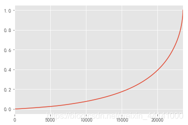
由图表可以看出,50%的用户仅仅贡献了15%的消费金额,而排名前20000的用户贡献了近40%的消费额。
3.用户消费行为
- 用户第一次消费时间分布(首购)
- 用户最后一次消费
- 新老客消费比
- 多少用户仅消费了一次?
- 每月新客占比?
- 用户分层
- RFM
- 新、活跃、回流、流失/不活跃
- 用户购买周期(按订单)
- 用户消费周期描述
- 用户消费周期分布
- 用户生命周期(按第一次和最后一次消费时间)
- 用户生命周期描述
- 用户生命周期分布
group_user['order_dt'].min().value_counts().plot()
<matplotlib.axes._subplots.AxesSubplot at 0xcabc7f0>
![]()
用户首购集中在前三个月,并且可以看出在第二月间有明显的波动
group_user['order_dt'].max().value_counts().plot()
<matplotlib.axes._subplots.AxesSubplot at 0xca506a0>
![]()
从图中可以看出,大部分用户在进行了第一次消费后就不再消费了,并且三月后,可以看出用户消费呈现不断流失的状态
多少用户仅消费了一次?
shop_time = group_user['order_dt'].agg(['min', 'max'])
shop_time.head()
| min | max | |
|---|---|---|
| user_id | ||
| 1 | 1997-01-01 | 1997-01-01 |
| 2 | 1997-01-12 | 1997-01-12 |
| 3 | 1997-01-02 | 1998-05-28 |
| 4 | 1997-01-01 | 1997-12-12 |
| 5 | 1997-01-01 | 1998-01-03 |
count = shop_time[shop_time['min']==shop_time['max']]
count.count()
min    12054
max    12054
dtype: int64
# 每月新客占比
month_user_sum = date.groupby('month')[['order_dt']].count()
month_user_sum = month_user_sum.cumsum()
user_class = date.groupby('user_id')
user_min = user_class.month.agg('min').reset_index()
user_min = user_min.groupby('month').count()
user_min
| user_id | |
|---|---|
| month | |
| 1997-01-01 | 7846 |
| 1997-02-01 | 8476 |
| 1997-03-01 | 7248 |
new_user = month_user_sum.join(user_min).fillna(0)
new_user
| order_dt | user_id | |
|---|---|---|
| month | ||
| 1997-01-01 | 8928 | 7846.0 |
| 1997-02-01 | 20200 | 8476.0 |
| 1997-03-01 | 31798 | 7248.0 |
| 1997-04-01 | 35579 | 0.0 |
| 1997-05-01 | 38474 | 0.0 |
| 1997-06-01 | 41528 | 0.0 |
| 1997-07-01 | 44470 | 0.0 |
| 1997-08-01 | 46790 | 0.0 |
| 1997-09-01 | 49086 | 0.0 |
| 1997-10-01 | 51648 | 0.0 |
| 1997-11-01 | 54398 | 0.0 |
| 1997-12-01 | 56902 | 0.0 |
| 1998-01-01 | 58934 | 0.0 |
| 1998-02-01 | 60960 | 0.0 |
| 1998-03-01 | 63753 | 0.0 |
| 1998-04-01 | 65631 | 0.0 |
| 1998-05-01 | 67616 | 0.0 |
| 1998-06-01 | 69659 | 0.0 |
def func_handel(x):return x.user_id / x.order_dt
new_user['proportion'] = new_user.apply(func_handel, axis=1).values
new_user
| order_dt | user_id | proportion | |
|---|---|---|---|
| month | |||
| 1997-01-01 | 8928 | 7846.0 | 0.878808 |
| 1997-02-01 | 20200 | 8476.0 | 0.419604 |
| 1997-03-01 | 31798 | 7248.0 | 0.227939 |
| 1997-04-01 | 35579 | 0.0 | 0.000000 |
| 1997-05-01 | 38474 | 0.0 | 0.000000 |
| 1997-06-01 | 41528 | 0.0 | 0.000000 |
| 1997-07-01 | 44470 | 0.0 | 0.000000 |
| 1997-08-01 | 46790 | 0.0 | 0.000000 |
| 1997-09-01 | 49086 | 0.0 | 0.000000 |
| 1997-10-01 | 51648 | 0.0 | 0.000000 |
| 1997-11-01 | 54398 | 0.0 | 0.000000 |
| 1997-12-01 | 56902 | 0.0 | 0.000000 |
| 1998-01-01 | 58934 | 0.0 | 0.000000 |
| 1998-02-01 | 60960 | 0.0 | 0.000000 |
| 1998-03-01 | 63753 | 0.0 | 0.000000 |
| 1998-04-01 | 65631 | 0.0 | 0.000000 |
| 1998-05-01 | 67616 | 0.0 | 0.000000 |
| 1998-06-01 | 69659 | 0.0 | 0.000000 |
将每月新客占比进行图的绘制
plt.plot(new_user.index, new_user.proportion)
plt.xticks(rotation=45)
plt.show()
![]()
从图中可以看出新客用户都集中在前三个月,并且每月新客占比逐月减少,到第三月后再无新增客户
rfm = date.pivot_table(index='user_id', values=['order_products','order_amount','order_dt'],aggfunc={'order_dt':'max','order_products':'sum','order_amount':'sum'})
rfm.head()
| order_amount | order_dt | order_products | |
|---|---|---|---|
| user_id | |||
| 1 | 11.77 | 1997-01-01 | 1 |
| 2 | 89.00 | 1997-01-12 | 6 |
| 3 | 156.46 | 1998-05-28 | 16 |
| 4 | 100.50 | 1997-12-12 | 7 |
| 5 | 385.61 | 1998-01-03 | 29 |
# -(rfm.order_dt - rfm.order_dt.max()) / np.timedelta64(1, 'D') # 将其转化为数字,而不是带着 days 的单位
rfm['R'] = -(rfm.order_dt - rfm.order_dt.max()) / np.timedelta64(1, 'D')
rfm.rename(columns={'order_products':'F','order_amount':'M'}, inplace=True)
rfm.head()
| M | order_dt | F | R | |
|---|---|---|---|---|
| user_id | ||||
| 1 | 11.77 | 1997-01-01 | 1 | 545.0 |
| 2 | 89.00 | 1997-01-12 | 6 | 534.0 |
| 3 | 156.46 | 1998-05-28 | 16 | 33.0 |
| 4 | 100.50 | 1997-12-12 | 7 | 200.0 |
| 5 | 385.61 | 1998-01-03 | 29 | 178.0 |
def rfm_func(x):level = x.apply(lambda x:'1' if x>=0 else '0')label = level.R + level.F + level.Md = {'111':'重要客户','011':'重要保持客户','101':'重要挽留客户','001':'重要发展客户','110':'一般客户','010':'一般保持客户','100':'一般挽留客户','000':'一般发展客户'}result = d[label]return result
rfm['label'] = rfm[['R','F','M']].apply(lambda x:x-x.mean()).apply(rfm_func, axis=1)
rfm.head()
| M | order_dt | F | R | label | |
|---|---|---|---|---|---|
| user_id | |||||
| 1 | 11.77 | 1997-01-01 | 1 | 545.0 | 一般挽留客户 |
| 2 | 89.00 | 1997-01-12 | 6 | 534.0 | 一般挽留客户 |
| 3 | 156.46 | 1998-05-28 | 16 | 33.0 | 重要保持客户 |
| 4 | 100.50 | 1997-12-12 | 7 | 200.0 | 一般发展客户 |
| 5 | 385.61 | 1998-01-03 | 29 | 178.0 | 重要保持客户 |
rfm.groupby('label').sum()
| M | F | R | |
|---|---|---|---|
| label | |||
| 一般保持客户 | 19937.45 | 1712 | 29448.0 |
| 一般发展客户 | 196971.23 | 13977 | 591108.0 |
| 一般客户 | 7181.28 | 650 | 36295.0 |
| 一般挽留客户 | 438291.81 | 29346 | 6951815.0 |
| 重要保持客户 | 1592039.62 | 107789 | 517267.0 |
| 重要发展客户 | 45785.01 | 2023 | 56636.0 |
| 重要客户 | 167080.83 | 11121 | 358363.0 |
| 重要挽留客户 | 33028.40 | 1263 | 114482.0 |
# 为相关的分组添加上标签
rfm.loc[rfm.label == '重要客户', 'color'] = 'g'
rfm.loc[~(rfm.label == '重要客户'), 'color'] = 'r'
rfm.plot.scatter('F','R',c=rfm.color)
<matplotlib.axes._subplots.AxesSubplot at 0xca0f908>
![]()
由RFM分层可得,大部分银行为重要保持客户,但这是由于极值的影响,所以RFM的划分标准应该以业务为准
- 尽量用小部分的用户涵盖大部分的额度
- 不要为了数据好看划分等级
# 新、活跃、回流、流失/不活跃
pivot_counts = date.pivot_table(index='user_id', columns='month', values='order_dt', aggfunc='count').fillna(0)
pivot_counts.head()
| month | 1997-01-01 00:00:00 | 1997-02-01 00:00:00 | 1997-03-01 00:00:00 | 1997-04-01 00:00:00 | 1997-05-01 00:00:00 | 1997-06-01 00:00:00 | 1997-07-01 00:00:00 | 1997-08-01 00:00:00 | 1997-09-01 00:00:00 | 1997-10-01 00:00:00 | 1997-11-01 00:00:00 | 1997-12-01 00:00:00 | 1998-01-01 00:00:00 | 1998-02-01 00:00:00 | 1998-03-01 00:00:00 | 1998-04-01 00:00:00 | 1998-05-01 00:00:00 | 1998-06-01 00:00:00 |
|---|---|---|---|---|---|---|---|---|---|---|---|---|---|---|---|---|---|---|
| user_id | ||||||||||||||||||
| 1 | 1.0 | 0.0 | 0.0 | 0.0 | 0.0 | 0.0 | 0.0 | 0.0 | 0.0 | 0.0 | 0.0 | 0.0 | 0.0 | 0.0 | 0.0 | 0.0 | 0.0 | 0.0 |
| 2 | 2.0 | 0.0 | 0.0 | 0.0 | 0.0 | 0.0 | 0.0 | 0.0 | 0.0 | 0.0 | 0.0 | 0.0 | 0.0 | 0.0 | 0.0 | 0.0 | 0.0 | 0.0 |
| 3 | 1.0 | 0.0 | 1.0 | 1.0 | 0.0 | 0.0 | 0.0 | 0.0 | 0.0 | 0.0 | 2.0 | 0.0 | 0.0 | 0.0 | 0.0 | 0.0 | 1.0 | 0.0 |
| 4 | 2.0 | 0.0 | 0.0 | 0.0 | 0.0 | 0.0 | 0.0 | 1.0 | 0.0 | 0.0 | 0.0 | 1.0 | 0.0 | 0.0 | 0.0 | 0.0 | 0.0 | 0.0 |
| 5 | 2.0 | 1.0 | 0.0 | 1.0 | 1.0 | 1.0 | 1.0 | 0.0 | 1.0 | 0.0 | 0.0 | 2.0 | 1.0 | 0.0 | 0.0 | 0.0 | 0.0 | 0.0 |
purchase_user = pivot_counts.applymap(lambda x:1 if x>0 else 0)
purchase_user.tail()
| month | 1997-01-01 00:00:00 | 1997-02-01 00:00:00 | 1997-03-01 00:00:00 | 1997-04-01 00:00:00 | 1997-05-01 00:00:00 | 1997-06-01 00:00:00 | 1997-07-01 00:00:00 | 1997-08-01 00:00:00 | 1997-09-01 00:00:00 | 1997-10-01 00:00:00 | 1997-11-01 00:00:00 | 1997-12-01 00:00:00 | 1998-01-01 00:00:00 | 1998-02-01 00:00:00 | 1998-03-01 00:00:00 | 1998-04-01 00:00:00 | 1998-05-01 00:00:00 | 1998-06-01 00:00:00 |
|---|---|---|---|---|---|---|---|---|---|---|---|---|---|---|---|---|---|---|
| user_id | ||||||||||||||||||
| 23566 | 0 | 0 | 1 | 0 | 0 | 0 | 0 | 0 | 0 | 0 | 0 | 0 | 0 | 0 | 0 | 0 | 0 | 0 |
| 23567 | 0 | 0 | 1 | 0 | 0 | 0 | 0 | 0 | 0 | 0 | 0 | 0 | 0 | 0 | 0 | 0 | 0 | 0 |
| 23568 | 0 | 0 | 1 | 1 | 0 | 0 | 0 | 0 | 0 | 0 | 0 | 0 | 0 | 0 | 0 | 0 | 0 | 0 |
| 23569 | 0 | 0 | 1 | 0 | 0 | 0 | 0 | 0 | 0 | 0 | 0 | 0 | 0 | 0 | 0 | 0 | 0 | 0 |
| 23570 | 0 | 0 | 1 | 0 | 0 | 0 | 0 | 0 | 0 | 0 | 0 | 0 | 0 | 0 | 0 | 0 | 0 | 0 |
def active_status(data):status = []for i in range(18):# 本月没有消费if data[i] == 0:if len(status) == 0:status.append('unregister')else:if status[i-1] == 'unregister':status.append('unregister')else:status.append('unactive')# 本月消费else:if len(status) == 0:status.append('new')else:if status[i-1] == 'unregister':status.append('new')elif status[i-1] == 'unactive':status.append('return')else:status.append('active')return status
purchase_user = purchase_user.apply(active_status, axis=1)
purchase_user.tail()
| month | 1997-01-01 00:00:00 | 1997-02-01 00:00:00 | 1997-03-01 00:00:00 | 1997-04-01 00:00:00 | 1997-05-01 00:00:00 | 1997-06-01 00:00:00 | 1997-07-01 00:00:00 | 1997-08-01 00:00:00 | 1997-09-01 00:00:00 | 1997-10-01 00:00:00 | 1997-11-01 00:00:00 | 1997-12-01 00:00:00 | 1998-01-01 00:00:00 | 1998-02-01 00:00:00 | 1998-03-01 00:00:00 | 1998-04-01 00:00:00 | 1998-05-01 00:00:00 | 1998-06-01 00:00:00 |
|---|---|---|---|---|---|---|---|---|---|---|---|---|---|---|---|---|---|---|
| user_id | ||||||||||||||||||
| 23566 | unregister | unregister | new | unactive | unactive | unactive | unactive | unactive | unactive | unactive | unactive | unactive | unactive | unactive | unactive | unactive | unactive | unactive |
| 23567 | unregister | unregister | new | unactive | unactive | unactive | unactive | unactive | unactive | unactive | unactive | unactive | unactive | unactive | unactive | unactive | unactive | unactive |
| 23568 | unregister | unregister | new | active | unactive | unactive | unactive | unactive | unactive | unactive | unactive | unactive | unactive | unactive | unactive | unactive | unactive | unactive |
| 23569 | unregister | unregister | new | unactive | unactive | unactive | unactive | unactive | unactive | unactive | unactive | unactive | unactive | unactive | unactive | unactive | unactive | unactive |
| 23570 | unregister | unregister | new | unactive | unactive | unactive | unactive | unactive | unactive | unactive | unactive | unactive | unactive | unactive | unactive | unactive | unactive | unactive |
purchase_user_status = purchase_user.replace('unregister', np.NaN).apply(lambda x:pd.value_counts(x))
purchase_user_status
| month | 1997-01-01 00:00:00 | 1997-02-01 00:00:00 | 1997-03-01 00:00:00 | 1997-04-01 00:00:00 | 1997-05-01 00:00:00 | 1997-06-01 00:00:00 | 1997-07-01 00:00:00 | 1997-08-01 00:00:00 | 1997-09-01 00:00:00 | 1997-10-01 00:00:00 | 1997-11-01 00:00:00 | 1997-12-01 00:00:00 | 1998-01-01 00:00:00 | 1998-02-01 00:00:00 | 1998-03-01 00:00:00 | 1998-04-01 00:00:00 | 1998-05-01 00:00:00 | 1998-06-01 00:00:00 |
|---|---|---|---|---|---|---|---|---|---|---|---|---|---|---|---|---|---|---|
| active | NaN | 1157.0 | 1681 | 1773.0 | 852.0 | 747.0 | 746.0 | 604.0 | 528.0 | 532.0 | 624.0 | 632.0 | 512.0 | 472.0 | 571.0 | 518.0 | 459.0 | 446.0 |
| new | 7846.0 | 8476.0 | 7248 | NaN | NaN | NaN | NaN | NaN | NaN | NaN | NaN | NaN | NaN | NaN | NaN | NaN | NaN | NaN |
| return | NaN | NaN | 595 | 1049.0 | 1362.0 | 1592.0 | 1434.0 | 1168.0 | 1211.0 | 1307.0 | 1404.0 | 1232.0 | 1025.0 | 1079.0 | 1489.0 | 919.0 | 1029.0 | 1060.0 |
| unactive | NaN | 6689.0 | 14046 | 20748.0 | 21356.0 | 21231.0 | 21390.0 | 21798.0 | 21831.0 | 21731.0 | 21542.0 | 21706.0 | 22033.0 | 22019.0 | 21510.0 | 22133.0 | 22082.0 | 22064.0 |
purchase_user_status.fillna(0).T
| active | new | return | unactive | |
|---|---|---|---|---|
| month | ||||
| 1997-01-01 | 0.0 | 7846.0 | 0.0 | 0.0 |
| 1997-02-01 | 1157.0 | 8476.0 | 0.0 | 6689.0 |
| 1997-03-01 | 1681.0 | 7248.0 | 595.0 | 14046.0 |
| 1997-04-01 | 1773.0 | 0.0 | 1049.0 | 20748.0 |
| 1997-05-01 | 852.0 | 0.0 | 1362.0 | 21356.0 |
| 1997-06-01 | 747.0 | 0.0 | 1592.0 | 21231.0 |
| 1997-07-01 | 746.0 | 0.0 | 1434.0 | 21390.0 |
| 1997-08-01 | 604.0 | 0.0 | 1168.0 | 21798.0 |
| 1997-09-01 | 528.0 | 0.0 | 1211.0 | 21831.0 |
| 1997-10-01 | 532.0 | 0.0 | 1307.0 | 21731.0 |
| 1997-11-01 | 624.0 | 0.0 | 1404.0 | 21542.0 |
| 1997-12-01 | 632.0 | 0.0 | 1232.0 | 21706.0 |
| 1998-01-01 | 512.0 | 0.0 | 1025.0 | 22033.0 |
| 1998-02-01 | 472.0 | 0.0 | 1079.0 | 22019.0 |
| 1998-03-01 | 571.0 | 0.0 | 1489.0 | 21510.0 |
| 1998-04-01 | 518.0 | 0.0 | 919.0 | 22133.0 |
| 1998-05-01 | 459.0 | 0.0 | 1029.0 | 22082.0 |
| 1998-06-01 | 446.0 | 0.0 | 1060.0 | 22064.0 |
purchase_user_status.fillna(0).T.plot.area()
<matplotlib.axes._subplots.AxesSubplot at 0xc9fc0b8>
![]()
purchase_user_status.fillna(0).T.apply(lambda x:x/x.sum(), axis=1)
| active | new | return | unactive | |
|---|---|---|---|---|
| month | ||||
| 1997-01-01 | 0.000000 | 1.000000 | 0.000000 | 0.000000 |
| 1997-02-01 | 0.070886 | 0.519299 | 0.000000 | 0.409815 |
| 1997-03-01 | 0.071319 | 0.307510 | 0.025244 | 0.595927 |
| 1997-04-01 | 0.075223 | 0.000000 | 0.044506 | 0.880272 |
| 1997-05-01 | 0.036148 | 0.000000 | 0.057785 | 0.906067 |
| 1997-06-01 | 0.031693 | 0.000000 | 0.067543 | 0.900764 |
| 1997-07-01 | 0.031650 | 0.000000 | 0.060840 | 0.907510 |
| 1997-08-01 | 0.025626 | 0.000000 | 0.049555 | 0.924820 |
| 1997-09-01 | 0.022401 | 0.000000 | 0.051379 | 0.926220 |
| 1997-10-01 | 0.022571 | 0.000000 | 0.055452 | 0.921977 |
| 1997-11-01 | 0.026474 | 0.000000 | 0.059567 | 0.913958 |
| 1997-12-01 | 0.026814 | 0.000000 | 0.052270 | 0.920916 |
| 1998-01-01 | 0.021723 | 0.000000 | 0.043487 | 0.934790 |
| 1998-02-01 | 0.020025 | 0.000000 | 0.045779 | 0.934196 |
| 1998-03-01 | 0.024226 | 0.000000 | 0.063174 | 0.912601 |
| 1998-04-01 | 0.021977 | 0.000000 | 0.038990 | 0.939033 |
| 1998-05-01 | 0.019474 | 0.000000 | 0.043657 | 0.936869 |
| 1998-06-01 | 0.018922 | 0.000000 | 0.044972 | 0.936105 |
由上表可知,每月用户消费状态变化
- 回流用户:之前没消费,本月才消费(唤回运营)
- 活跃用户:持续消费(消费运营的质量)
- 不活跃用户:流失用户
# 用户购买周期(按订单)    shift()函数是使得数据矩阵偏移一个单位
order_diff = group_user.apply(lambda x:(x.order_dt - x.order_dt.shift()) / np.timedelta64(1, 'D'))
order_diff.hist(bins=20)
<matplotlib.axes._subplots.AxesSubplot at 0x1299db00>
![]()
# 用户生命周期(按第一次和最后一次消费时间)
user_period = group_user.order_dt.agg(['max', 'min'])
user_period = user_period.apply(lambda x:(x['max'] - x['min']) / np.timedelta64(1, 'D'), axis=1)
user_period.describe()
count    23570.000000
mean       134.871956
std        180.574109
min          0.000000
25%          0.000000
50%          0.000000
75%        294.000000
max        544.000000
dtype: float64
user_period = pd.DataFrame(user_period, columns=['diff'])
user_period.head()
| diff | |
|---|---|
| user_id | |
| 1 | 0.0 |
| 2 | 0.0 |
| 3 | 511.0 |
| 4 | 345.0 |
| 5 | 367.0 |
user_period[user_period['diff']!=0].hist(bins=40) # 将生命周期为0的全部剔除掉
array([[<matplotlib.axes._subplots.AxesSubplot object at 0x000000000B3A2DD8>]], dtype=object)
![]()
复购率和回购率分析
- 复购率
- 自然月内,购买多次的用户占比
- 回购率
- 曾经购买过的用户在某一段时间内的再次购买的占比
pivot_counts.head(10)
| month | 1997-01-01 00:00:00 | 1997-02-01 00:00:00 | 1997-03-01 00:00:00 | 1997-04-01 00:00:00 | 1997-05-01 00:00:00 | 1997-06-01 00:00:00 | 1997-07-01 00:00:00 | 1997-08-01 00:00:00 | 1997-09-01 00:00:00 | 1997-10-01 00:00:00 | 1997-11-01 00:00:00 | 1997-12-01 00:00:00 | 1998-01-01 00:00:00 | 1998-02-01 00:00:00 | 1998-03-01 00:00:00 | 1998-04-01 00:00:00 | 1998-05-01 00:00:00 | 1998-06-01 00:00:00 |
|---|---|---|---|---|---|---|---|---|---|---|---|---|---|---|---|---|---|---|
| user_id | ||||||||||||||||||
| 1 | 1.0 | 0.0 | 0.0 | 0.0 | 0.0 | 0.0 | 0.0 | 0.0 | 0.0 | 0.0 | 0.0 | 0.0 | 0.0 | 0.0 | 0.0 | 0.0 | 0.0 | 0.0 |
| 2 | 2.0 | 0.0 | 0.0 | 0.0 | 0.0 | 0.0 | 0.0 | 0.0 | 0.0 | 0.0 | 0.0 | 0.0 | 0.0 | 0.0 | 0.0 | 0.0 | 0.0 | 0.0 |
| 3 | 1.0 | 0.0 | 1.0 | 1.0 | 0.0 | 0.0 | 0.0 | 0.0 | 0.0 | 0.0 | 2.0 | 0.0 | 0.0 | 0.0 | 0.0 | 0.0 | 1.0 | 0.0 |
| 4 | 2.0 | 0.0 | 0.0 | 0.0 | 0.0 | 0.0 | 0.0 | 1.0 | 0.0 | 0.0 | 0.0 | 1.0 | 0.0 | 0.0 | 0.0 | 0.0 | 0.0 | 0.0 |
| 5 | 2.0 | 1.0 | 0.0 | 1.0 | 1.0 | 1.0 | 1.0 | 0.0 | 1.0 | 0.0 | 0.0 | 2.0 | 1.0 | 0.0 | 0.0 | 0.0 | 0.0 | 0.0 |
| 6 | 1.0 | 0.0 | 0.0 | 0.0 | 0.0 | 0.0 | 0.0 | 0.0 | 0.0 | 0.0 | 0.0 | 0.0 | 0.0 | 0.0 | 0.0 | 0.0 | 0.0 | 0.0 |
| 7 | 1.0 | 0.0 | 0.0 | 0.0 | 0.0 | 0.0 | 0.0 | 0.0 | 0.0 | 1.0 | 0.0 | 0.0 | 0.0 | 0.0 | 1.0 | 0.0 | 0.0 | 0.0 |
| 8 | 1.0 | 1.0 | 0.0 | 0.0 | 0.0 | 1.0 | 1.0 | 0.0 | 0.0 | 0.0 | 2.0 | 1.0 | 0.0 | 0.0 | 1.0 | 0.0 | 0.0 | 0.0 |
| 9 | 1.0 | 0.0 | 0.0 | 0.0 | 1.0 | 0.0 | 0.0 | 0.0 | 0.0 | 0.0 | 0.0 | 0.0 | 0.0 | 0.0 | 0.0 | 0.0 | 0.0 | 1.0 |
| 10 | 1.0 | 0.0 | 0.0 | 0.0 | 0.0 | 0.0 | 0.0 | 0.0 | 0.0 | 0.0 | 0.0 | 0.0 | 0.0 | 0.0 | 0.0 | 0.0 | 0.0 | 0.0 |
re_purchase = pivot_counts.applymap(lambda x:1 if x>1 else np.NaN if x==0 else 0)
re_purchase.head(10)
| month | 1997-01-01 00:00:00 | 1997-02-01 00:00:00 | 1997-03-01 00:00:00 | 1997-04-01 00:00:00 | 1997-05-01 00:00:00 | 1997-06-01 00:00:00 | 1997-07-01 00:00:00 | 1997-08-01 00:00:00 | 1997-09-01 00:00:00 | 1997-10-01 00:00:00 | 1997-11-01 00:00:00 | 1997-12-01 00:00:00 | 1998-01-01 00:00:00 | 1998-02-01 00:00:00 | 1998-03-01 00:00:00 | 1998-04-01 00:00:00 | 1998-05-01 00:00:00 | 1998-06-01 00:00:00 |
|---|---|---|---|---|---|---|---|---|---|---|---|---|---|---|---|---|---|---|
| user_id | ||||||||||||||||||
| 1 | 0.0 | NaN | NaN | NaN | NaN | NaN | NaN | NaN | NaN | NaN | NaN | NaN | NaN | NaN | NaN | NaN | NaN | NaN |
| 2 | 1.0 | NaN | NaN | NaN | NaN | NaN | NaN | NaN | NaN | NaN | NaN | NaN | NaN | NaN | NaN | NaN | NaN | NaN |
| 3 | 0.0 | NaN | 0.0 | 0.0 | NaN | NaN | NaN | NaN | NaN | NaN | 1.0 | NaN | NaN | NaN | NaN | NaN | 0.0 | NaN |
| 4 | 1.0 | NaN | NaN | NaN | NaN | NaN | NaN | 0.0 | NaN | NaN | NaN | 0.0 | NaN | NaN | NaN | NaN | NaN | NaN |
| 5 | 1.0 | 0.0 | NaN | 0.0 | 0.0 | 0.0 | 0.0 | NaN | 0.0 | NaN | NaN | 1.0 | 0.0 | NaN | NaN | NaN | NaN | NaN |
| 6 | 0.0 | NaN | NaN | NaN | NaN | NaN | NaN | NaN | NaN | NaN | NaN | NaN | NaN | NaN | NaN | NaN | NaN | NaN |
| 7 | 0.0 | NaN | NaN | NaN | NaN | NaN | NaN | NaN | NaN | 0.0 | NaN | NaN | NaN | NaN | 0.0 | NaN | NaN | NaN |
| 8 | 0.0 | 0.0 | NaN | NaN | NaN | 0.0 | 0.0 | NaN | NaN | NaN | 1.0 | 0.0 | NaN | NaN | 0.0 | NaN | NaN | NaN |
| 9 | 0.0 | NaN | NaN | NaN | 0.0 | NaN | NaN | NaN | NaN | NaN | NaN | NaN | NaN | NaN | NaN | NaN | NaN | 0.0 |
| 10 | 0.0 | NaN | NaN | NaN | NaN | NaN | NaN | NaN | NaN | NaN | NaN | NaN | NaN | NaN | NaN | NaN | NaN | NaN |
re_purchase.apply(lambda x:x.sum()/x.count()).plot(figsize=(10, 4))
<matplotlib.axes._subplots.AxesSubplot at 0x28a1390>
![]()
复购率在前三月增长的较快,可能是新增用户基数较大,但大部分都是只购买了一次,导致复购率较低,随后一直稳定在20%左右
# 回购率是指本月消费了的用户中,在下一月继续消费的用户有多少
repurchase = pivot_counts.applymap(lambda x:1 if x>0 else  0)
repurchase.head(10)
| month | 1997-01-01 00:00:00 | 1997-02-01 00:00:00 | 1997-03-01 00:00:00 | 1997-04-01 00:00:00 | 1997-05-01 00:00:00 | 1997-06-01 00:00:00 | 1997-07-01 00:00:00 | 1997-08-01 00:00:00 | 1997-09-01 00:00:00 | 1997-10-01 00:00:00 | 1997-11-01 00:00:00 | 1997-12-01 00:00:00 | 1998-01-01 00:00:00 | 1998-02-01 00:00:00 | 1998-03-01 00:00:00 | 1998-04-01 00:00:00 | 1998-05-01 00:00:00 | 1998-06-01 00:00:00 |
|---|---|---|---|---|---|---|---|---|---|---|---|---|---|---|---|---|---|---|
| user_id | ||||||||||||||||||
| 1 | 1 | 0 | 0 | 0 | 0 | 0 | 0 | 0 | 0 | 0 | 0 | 0 | 0 | 0 | 0 | 0 | 0 | 0 |
| 2 | 1 | 0 | 0 | 0 | 0 | 0 | 0 | 0 | 0 | 0 | 0 | 0 | 0 | 0 | 0 | 0 | 0 | 0 |
| 3 | 1 | 0 | 1 | 1 | 0 | 0 | 0 | 0 | 0 | 0 | 1 | 0 | 0 | 0 | 0 | 0 | 1 | 0 |
| 4 | 1 | 0 | 0 | 0 | 0 | 0 | 0 | 1 | 0 | 0 | 0 | 1 | 0 | 0 | 0 | 0 | 0 | 0 |
| 5 | 1 | 1 | 0 | 1 | 1 | 1 | 1 | 0 | 1 | 0 | 0 | 1 | 1 | 0 | 0 | 0 | 0 | 0 |
| 6 | 1 | 0 | 0 | 0 | 0 | 0 | 0 | 0 | 0 | 0 | 0 | 0 | 0 | 0 | 0 | 0 | 0 | 0 |
| 7 | 1 | 0 | 0 | 0 | 0 | 0 | 0 | 0 | 0 | 1 | 0 | 0 | 0 | 0 | 1 | 0 | 0 | 0 |
| 8 | 1 | 1 | 0 | 0 | 0 | 1 | 1 | 0 | 0 | 0 | 1 | 1 | 0 | 0 | 1 | 0 | 0 | 0 |
| 9 | 1 | 0 | 0 | 0 | 1 | 0 | 0 | 0 | 0 | 0 | 0 | 0 | 0 | 0 | 0 | 0 | 0 | 1 |
| 10 | 1 | 0 | 0 | 0 | 0 | 0 | 0 | 0 | 0 | 0 | 0 | 0 | 0 | 0 | 0 | 0 | 0 | 0 |
def Repurchase(data):is_purchase = []for i in range(0, 17):# 本月消费了if data[i] > 0:# 下月消费了if data[i+1] > 0:is_purchase.append(1)# 下月没有消费else:is_purchase.append(0)# 本月没有消费else:# 不管下月消费与否is_purchase.append(np.NaN)is_purchase.append(np.NaN)return is_purchase
repurchase = repurchase.apply(Repurchase, axis=1)
repurchase.head(5)
| month | 1997-01-01 00:00:00 | 1997-02-01 00:00:00 | 1997-03-01 00:00:00 | 1997-04-01 00:00:00 | 1997-05-01 00:00:00 | 1997-06-01 00:00:00 | 1997-07-01 00:00:00 | 1997-08-01 00:00:00 | 1997-09-01 00:00:00 | 1997-10-01 00:00:00 | 1997-11-01 00:00:00 | 1997-12-01 00:00:00 | 1998-01-01 00:00:00 | 1998-02-01 00:00:00 | 1998-03-01 00:00:00 | 1998-04-01 00:00:00 | 1998-05-01 00:00:00 | 1998-06-01 00:00:00 |
|---|---|---|---|---|---|---|---|---|---|---|---|---|---|---|---|---|---|---|
| user_id | ||||||||||||||||||
| 1 | 0.0 | NaN | NaN | NaN | NaN | NaN | NaN | NaN | NaN | NaN | NaN | NaN | NaN | NaN | NaN | NaN | NaN | NaN |
| 2 | 0.0 | NaN | NaN | NaN | NaN | NaN | NaN | NaN | NaN | NaN | NaN | NaN | NaN | NaN | NaN | NaN | NaN | NaN |
| 3 | 0.0 | NaN | 1.0 | 0.0 | NaN | NaN | NaN | NaN | NaN | NaN | 0.0 | NaN | NaN | NaN | NaN | NaN | 0.0 | NaN |
| 4 | 0.0 | NaN | NaN | NaN | NaN | NaN | NaN | 0.0 | NaN | NaN | NaN | 0.0 | NaN | NaN | NaN | NaN | NaN | NaN |
| 5 | 1.0 | 0.0 | NaN | 1.0 | 1.0 | 1.0 | 0.0 | NaN | 0.0 | NaN | NaN | 1.0 | 0.0 | NaN | NaN | NaN | NaN | NaN |
repurchase.apply(lambda x:x.sum()/x.count()).plot(figsize=(10,4))
D:\Anaconda3\lib\site-packages\ipykernel_launcher.py:1: RuntimeWarning: invalid value encountered in true_divide"""Entry point for launching an IPython kernel.<matplotlib.axes._subplots.AxesSubplot at 0xaad40b8>
![]()
用户购买CD行为数据分析相关推荐
- 用户购买CD消费行为分析
用户购买CD消费行为分析 1.进行用户消费趋势的分析(按月) 1.1每月的消费总金额 1.2每月的消费次数 1.3每月的产品购买量 1.4每月的消费人数 2.用户个体消费分析 2.1用户消费金额.消费 ...
- 用pandas进行数据分析:结合JData ”用户购买时间预测“数据分析实例(三)
表3:用户行为表(jdata_user_action) 1. 读取数据,并获取数据基本信息 2. 获取部分特征的频率统计和最大/最小值 3. 获取行为次数的统计
- 天猫用户重复购买预测之数据分析
赛题理解 赛题链接 赛题背景: 商家有时会在特定日期,例如Boxing-day,黑色星期五或是双十一(11月11日)开展大型促销活动或者发放优惠券以吸引消费者,然而很多被吸引来的买家都是一次性消费者, ...
- php汽车购买意向调查,2012年中国汽车用户购买意向调查报告(已购汽车篇)
近年来,随着国民生活质量的日渐提高,汽车已经逐渐成为普通家庭日常生活的必需品,越来越多的消费者开始考虑购买属于自己的汽车.为了更好了解中国消费者对于汽车的消费需求,互联网消费调研中心ZDC进行了本次调 ...
- JData数据处理及高潜用户购买意向预测
竞赛概述: 本次大赛以京东商城真实的用户.商品和行为数据(脱敏后)为基础,参赛队伍需要通过数据挖掘的技术和机器学习的算法,构建用户购买商品的预测模型,输出高潜用户和目标商品的匹配结果,为精准营销提供高 ...
- 32销售是合理的引导用户购买
销售一定是合理的去引导用户,如果不进行合理的引导,那么在用户的面前,这件事很可能觉得莫名其妙. 对于一个产品任何一个用户都是陌生的,无论是否有这种需要,他都是陌生的,这个陌生来自于对使用的陌生.对该产 ...
- oracle:用户购买平台案例分析与优化
用户购买平台案例,涉及时间型数据.个人第一眼感觉特别简单,但是当深入处理是难成狗了.虽然在测试样例中的结果中通过,但是在最终提交过程中,却显示超时.唉,还得优化呀!本文就是关于这个问题的分析和总结. ...
- 操作系统的不确定性是指程序执行结果的不确定性_用不确定性促销策略提高用户购买意愿...
本文作者整理了关于不确定性促销策略的相关问题,结合案例对其一一展开了分析探究. 一.前言 促销玩法是电商运营的重要组成部分,我们整理了目前有关不确定性促销策略的前沿学术研究成果,希望以此解答以下问题, ...
- Java初学者作业——编写Java程序, 实现根据用户购买商品总金额, 计算实际支付的金额及所获得的购物券金额。
返回本章节 返回作业目录 需求说明: 编写Java程序, 实现根据用户购买商品总金额, 计算实际支付的金额及所获得的购物券金额. 购买总金额达到或超过 1000元,按 8折优惠,送 200元的购物券: ...
最新文章
- 命令行避免输入错误文件名_GitHub 60000+ Star 登顶,命令行的艺术
- Exchange 2007迁移Exchange 2010应该注意的13件事
- 同网段DHCP配置实验
- 学习共享--产品思维
- mysql 导入导出 备份_MySQL - 数据备份与还原(导出导入)
- [2018.10.11 T2] 整除
- SQLServer常用SQL语句
- 网络安全实验四 防火墙技术的具体应用
- 经济应用文写作【10】
- mui如何对接java后台_MUI框架-09-MUI 与后台数据交互
- C++优先级队列priority_queue详解及其模拟实现
- 抗洪救灾,共克时艰,城联优品捐赠10万元爱心物资驰援英德
- CentOS cowsay “会说话的小动物”
- 从C到B,20岁的腾讯正在经历一场“生死”腾挪
- 世界杯期间怎么做营销活动?
- 乳腺癌诊断和药物技术行业调研报告 - 市场现状分析与发展前景预测
- 【000】欢迎来到嵌入式开发教程
- 口嫌体正直,“苹果”们纷纷下场造车
- 三坐标最小二乘法原理_全最小二乘法在三坐标测量中的应用
- 骚操作!用Python自动下载抖音小姐姐