Haar Wavelet Transformation

原文转载自：http://www.whydomath.org/node/wavlets/hwt.html

Introduction

The easiest of all discrete wavelet transformations is the Discrete Haar Wavelet Tranformation (HWT). Let's motivate it's construction with the following example:

Suppose you had the eight numbers 100, 200, 44, 50, 20, 20, 4, 2 (these could be grayscale intensities) and you wanted to send an approximation of the list to a friend. Due to bandwidth constraints (this is a really old system!), you are only allowed to send your friend four values. What four values would you send your friend that might represent an approximation of the eight given values?

There are obviously many possible answers to this question, but one of the most common solutions is to take the eight numbers, two at a time, and average them. This computation would produce the four values 150, 47, 20, and 3. This list would represent an approximation to the original eight values.

Unfortunately, if your friend receives the four values 150, 47, 20, and 3, she has no chance of producing the original eight values from them - more information is needed. Suppose you are allowed to send an additional four values to your friend. With these values and the first four values, she should be able to reconstruct your original list of eight values. What values would you send her?

Suppose we sent our friend the values 50, 3, 0, and -1. How did we arrive at these values? They are simply the directed distances from the pairwise average to the second number in each pair: 150 + 50 = 200, 47 + 3 = 50, 20 + 0 = 20, and 3 + (-1) = 2. Note that if we subtract the values in this list from the pairwise averages, we arrive at the first number in each pair: 150 - 50 = 100, 47 - 3 = 44, 20 - 0 = 20, and 3 - (-1) = 4. So with the lists (150,47,20,3) and (50,3,0,-1), we can completely reconstruct the original list (100,200,44,50,20,20,4,2).

Given two numbers a and b, we have the following transformation:

(a, b) ( (b + a)/2, (b - a)/2 )

We will call the first output the average and the second output the difference.

So why would we consider sending (150,47,20,3 | 50, 3, 0, -1) instead of (100,200,44,50,20,20,4,2)? Two reasons quickly come to mind. The differences in the transformed list tell us about the trends in the data - big differences indicate large jumps between values while small values tell us that there is relatively little change in that portion of the input. Also, if we are interested in lossy compression, then small differences can be converted to zero and in this way we can improve the efficiency of the coder. Suppose we converted the last three values of the transformation to zero. Then we would transmit (150, 47, 20, 3 | 50, 0, 0, 0). The recipient could invert the process and obtain the list

(150-50, 150+50, 47-3, 47+3, 20-0, 20+0, 3-0, 3+0) = (100,200,44,50,20,20,3,3)

The "compressed" list is very similar to the original list!

Matrix Formulation

For an even-length list (vector) of numbers, we can also form a matrix product that computes this transformation. For the sake of illustration, let's assume our list (vector) is length 8. If we put the averages as the first half of the output and differences as the second half of the output, then we have the following matrix product:

W8v= 12 0 0 0 −12 0 0 0 12 0 0 0 12 0 0 0 0 12 0 0 0 −12 0 0 0 12 0 0 0 12 0 0 0 0 12 0 0 0 −12 0 0 0 12 0 0 0 12 0 0 0 0 12 0 0 0 −12 0 0 0 12 0 0 0 12 v1 v2 v3 v4 v5 v6 v7 v8 = (v1+v2)2 (v3+v4)2 (v5+v6)2 (v7+v8)2 (v2−v1)2 (v4−v3)2 (v6−v5)2 (v8−v7)2 =y

Inverting the Process

Inverting is easy - if we subtract y5 from y1, we obtain v1 . If we add y5 and y1, we obtain v2 . We can continue in a similar manner adding and subtracting pairs to completely recover v . We can also write the inverse process as a matrix product. We have:

W8−1y= 1 1 0 0 0 0 0 0 0 0 1 1 0 0 0 0 0 0 0 0 1 1 0 0 0 0 0 0 0 0 1 1 −1 1 0 0 0 0 0 0 0 0 −1 1 0 0 0 0 0 0 0 0 −1 1 0 0 0 0 0 0 0 0 −1 1 (v1+v2)2 (v3+v4)2 (v5+v6)2 (v7+v8)2 (v2−v1)2 (v4−v3)2 (v6−v5)2 (v8−v7)2 = v1 v2 v3 v4 v5 v6 v7 v8 =v

The matrix W8 satisfies another interesting property - we can compute the inverse by doubling the transpose! That is,

W8−1=2W8T

For those of you who have taken a linear algebra course, you may remember that orthogonal matrices U satisfyU−1=UT . We almost have that with our transformation. Indeed if we construct W8=2W8 , we have

W8−1 = = = = = = (2W8)−1 (12)W8−1 (12)2W8T 2W8T (2W8T)T W8T

Haar Wavelet Transform Defined

We will define the HWT as the orthogonal matrix described above. That is, for N even, the Discrete Haar Wavelet Transformation is defined as

WN= 22 0 0 −22 0 0 22 0 0 22 0 0 0 22 0 0 −22 0 0 22 0 0 22 0 0 0 22 0 0 −22 0 0 22 0 0 22

and the inverse HWT is WN−1=WNT.

Analysis of the HWT

The first N/2 rows of the HWT produce a weighted average of the input list taken two at a time. The weight factor is 2 . The last N/2 row of the HWT produce a weighted difference of the input list taken two at a time. The weight factor is also 2 .

We define the Haar filter as the numbers used to form the first row of the transform matrix. That is, the Haar filter is h=h0h1=2222 . This filter is also called a lowpass filter - since it averages pairs of numbers, it tends to reproduce (modulo the 2 ) two values that are similar and send to 0 to numbers that are (near) opposites of each other. Note also that the sum of the filter values is 2 .

We call the filter that is used to build the bottom half of the HWT a highpass filter. In this case, we have g=g0g1=−2222 . Highpass filters process data exactly opposite of lowpass filters. If two numbers are near in value, the highpass filter will return a value near zero. If two numbers are (near) opposites of each other, then the highpass filter will return a weighted version of one of the two numbers.

Fourier Series From the Filters

An important tool for constructing filters for discrete wavelet transformations is Fourier series. To analyze a given filter h=(h0h1h2hL) , engineers will use the coefficients to form a Fourier series

H()=h0+h1ei+h2e2i++hLeLi

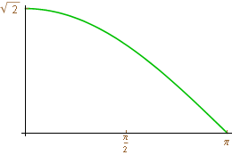
and then plot the absolute value of this series. It turns out that we can identify lowpass filters and highpass filters from these graphs. The plots for the filters for the HWT H()=22+22ei and G()=−22+22ei appear below:


		H()			G()

Note that the first graph has value 2 at 0 and H()=0. The graph for the highpass filter is just the opposite -G(0)=0 and G()=2 . This is typical of lowpass and highpass filters. We can also put other conditions on these graphs and that is often how more sophisticated lowpass/highpass filter pairs for the DWT are defined.

HWT and Digital Images

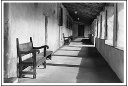
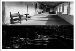
How do we apply the HWT to a digital grayscale image? If the image is stored in matrix A with even dimensions M x N, then the natural thing to try is to compute WMA . We can view this matrix multiplication as WM applied to each column of A so the output should be an M x N matrix where each column is M/2 weighted averages followed by M/2 weighted differences. The plots below illustrate the process:


		A digital image. Fullsize version			W160A . Fullsize version

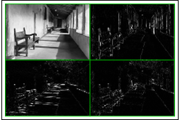
We have used the Haar matrix to process the columns of image matrix A. It is desirable to process the rows of the image as well. We proceed by multiplying WMA on the right by WNT. Transposing the wavelet matrix puts the filter coefficients in the columns and multiplication on the right by WNT means that we will be dotting the rows of WMA with the columns of WNT (columns of WN ). So the two dimensional HWT is defined as:

B=WMAWNT

The process is illustrated below.


		The two-dimensional HWT. Fullsize version

Analysis of the Two-Dimensional HWT

You can see why the wavelet transformation is well-suited for image compression. The two-dimensional HWT of the image has most of the energy conserved in the upper left-hand corner of the transform - the remaining three-quarters of the HWT consists primarily of values that are zero or near zero. The transformation is local as well - it turns out any element of the HWT is constructed from only four elements of the original input image. If we look at the HWT as a block matrix product, we can gain further insight about the transformation.

Suppose that the input image is square so we will drop the subscripts that indicate the dimension of the HWT matrix. If we use H to denote the top block of the HWT matrix and G to denote the bottom block of the HWT, we can express the transformation as:

B=WAWT=H G AH G T=H G AHT GT =HA GA HT GT =HAHT GAHT HAGT GAGT

We now see why there are four blocks in the wavelet transform. Let's look at each block individually. Note that the matrix H is constructed from the lowpass Haar filter and computes weighted averages while G computes weighted differences.

The upper left-hand block is HAHT - HA averages columns of A and the rows of this product are averaged by multiplication with HT. Thus the upper left-hand corner is an approximation of the entire image. In fact, it can be shown that elements in the upper left-hand corner of the HWT can be constructed by computing weighted averages of each 2 x 2 block of the input matrix. Mathematically, the mapping is

a c b d 2 ( a + b + c + d )/4

The upper right-hand block is HAGT - HA averages columns of A and the rows of this product are differenced by multiplication with GT. Thus the upper right-hand corner holds information about vertical in the image - large values indicate a large vertical change as we move across the image and small values indicate little vertical change. Mathematically, the mapping is

a c b d 2 ( b + d - a - c)/4

The lower left-hand block is GAHT - GA differences columns of A and the rows of this product are averaged by multiplication with HT. Thus the lower left-hand corner holds information about horizontal in the image - large values indicate a large horizontal change as we move down the image and small values indicate little horizontal change. Mathematically, the mapping is

a c b d 2 ( c + d - a - b )/4

The lower right-hand block is differences across both columns and rows and the result is a bit harder to see. It turns out that this product measures changes along 45-degree lines. This is diagonal differences. Mathematically, the mapping is

a c b d 2 ( b + c - a - d )/4

To summarize, the HWT of a digital image produces four blocks. The upper-left hand corner is an approximation or blur of the original image. The upper-right, lower-left, and lower-right blocks measure the differences in the vertical, horizontal, and diagonal directions, respectively.

Iterating the Process

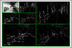
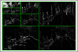
If there is not much change in the image, the difference blocks are comprised of (near) zero values. If we apply quantization and convert near-zero values to zero, then the HWT of the image can be effectively coded and the storage space for the image can be drastically reduced. We can iterate the HWT and produce an even better result to pass to the coder. Suppose we compute the HWT of a digital image. Most of the high intensities are contained in the blur portion of the transformation. We can iterate and apply the HWT to the blur portion of the transform. So in the composite transformation, we replace the blur by its transformation! The process is completely invertible - we apply the inverse HWT to the transform of the blur to obtain the blur. Then we apply the inverse HWT to obtain the original image. We can continue this process as often as we desire (and provided the dimensions of the data are divisible by suitable powers of two). The illustrations below show two iterations and three iterations of the HWT.


		Two iterations of the HWT. Fullsize version			Three iterations of the HWT Fullsize version


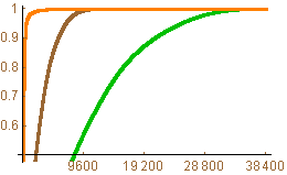
		Energy distribution for the image and HWTs.

The iterated HWT is an effective tool for conserving the energy of a digital image. The plot below shows the energy distribution for the original image (green), one iteration of the HWT (brown), and three iterations of the HWT (orange). The horizontal scale is pixels (there are 38,400 pixels in the thumbnail of the image). For a given pixel value p, the height represents the percentage of energy stored in the largest p pixels of the image. Note that the HWT gets to 1 (100% of the energy) much faster than the original image and the iterated HWT is much better than either the HWT or the original image.

Summary

The HWT is a wonderful tool for understanding how a discrete wavelet tranformation works. It is not desirable in practice because the filters are too short - since each filter is length two, the HWT decouples the data to create values of the transform. In particular, each value of the transform is created from a 2 x 2 block from the original input. If there is a large change between say row 6 and row 7, the HWT will not detect it. The HWT also send integers to irrational numbers and for lossless image compression, it is crucial that the transform send integers to integers. For these reasons, researchers developed more sophisticated filters. Be sure to check out the other subsections to learn more other types of wavelet filters.