Colab notebook, Github

Colab笔记本 ， Github

动机：最佳控制 (Motivation: Optimal Control)

Control systems are found everywhere, ranging from nuclear reactors to self driving cars. They react to a variety of scenarios while optimizing a set of often conflicting objectives. For example, autonomous vehicles seek to take you from A to B quickly while still ensuring safety and minimizing energy usage. These problems go by a variety of names. The AI & data science crowd calls it autonomy and reinforcement learning while engineers traditionally called it optimal control, state feedback control, model predictive control… The former tends to emphasize discrete actions in a complex changing environment while the later is associated with continuous signal actuation in a fixed industrial process. Advancement in control systems have taken us from the industrial revolution to the dawn of robotic autonomy.

控制系统无处不在，从核React堆到自动驾驶汽车。 他们对各种情况做出React，同时优化了一组经常相互矛盾的目标。 例如，自动驾驶汽车试图Swift将您从A带到B，同时仍要确保安全并最大程度地减少能耗。 这些问题有各种各样的名字。 AI和数据科学界将其称为自主性和强化学习，而工程师传统上将其称为最佳控制，状态反馈控制，模型预测控制……前者倾向于在复杂变化的环境中强调离散动作，而后者则与连续信号激励相关。固定的工业过程。 控制系统的进步已将我们从工业革命带到了机器人自治的曙光。

背景：为什么使用神经ODE？ (Background: Why Neural ODEs?)

Optimally controlling complex systems requires nonlinear response functions to the state variables. Thus we use neural networks as the controller (agent). Next, to model continuous time system dynamics, we use ODEs. Thus, neural + ODE :)

优化控制复杂系统需要对状态变量进行非线性响应。 因此，我们使用神经网络作为控制器(代理)。 接下来，为了对连续时间系统动力学建模，我们使用ODE。 因此，神经+ ODE :)

Actually I didn’t coin the term :) Neural ODEs were first popularized in the 2018 paper “Neural Ordinary Differential Equations,” winning the best paper award at the prestigious NIPS conference. The idea is simple: use a neural network instead to compute the derivative for an ODE. The original paper used it to approximate residual connections in discrete neural networks. However, we use it in the literal sense to model time evolving systems. We train the “neural” part of the neural ODE to be our agent or controller while the system evolves as a function of its state variables and the control signal. Surprisingly, this offers an elegant and practical formulation for a wide range of problems in reinforcement learning and optimal control.

其实我没有硬币术语:)神经微分方程最初是在2018年纸推广“ 神经常微分方程 ”，并获得了著名的NIPS会议的最佳论文奖。 这个想法很简单：使用神经网络代替来计算ODE的导数。 原始论文使用它来近似离散神经网络中的残余连接。 但是，我们从字面意义上使用它来建模时间演化系统。 我们训练神经ODE的“神经”部分作为我们的代理或控制器，而系统则根据其状态变量和控制信号进行演化。 令人惊讶的是，这为强化学习和最佳控制中的各种问题提供了一种优雅而实用的公式。

方法 (Method)

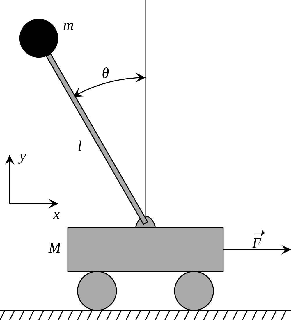
We tackle the “Hello World” of reinforcement learning and optimal control: the cartpole problem. The usual goal is to balance an upright pole by moving the base cart. This is actually too easy because the system is fairly linear at small angles :) Instead, we’ll start the pole hanging down and then compute the base movements to bring it up and balanced, aka cartpole swing up. This sweeps through the system’s nonlinearities. We wish to minimize the angle, angular velocity, and cart velocity in the end while staying within a time limit.

我们处理强化学习和最佳控制的“ Hello World”：难题。 通常的目标是通过移动底座推车来平衡立杆。 这实际上太容易了，因为系统在很小的角度上是线性的：)相反，我们将杆垂下，然后计算基本运动以使其上升并保持平衡，也就是使杆摆动。 这席卷了系统的非线性。 我们希望最终将角度，角速度和手推车速度最小化，同时保持在一个时间限制内。

The System (Environment) is the cartpole, while the Controller (Agent) dictates how to move the cart. The time derivative f of the system state vector x describes its time evolution. It’s a function of its current state and the control action. We make the controller a neural network g(x, p) with the system state x as input, p as parameters, and force to be applied to the cart as output. Goal is to optimize g wrt p.

系统(环境)是Struts，而控制器(代理人)则指示如何移动推车。 系统状态向量x的时间导数f描述其时间演化。 它是其当前状态和控制动作的函数。 我们使控制器成为神经网络g ( x，p ) 系统状态x为输入， p为参数，而要施加到手推车的力为输出。 目标是优化g wrt p 。

We use Julia, a modern language similar to Python but with easier and more performant syntax for scientific computing. Think of it as a happy marriage between Python, R, Matlab, and C++.

我们使用Julia，这是一种类似于Python的现代语言，但具有用于科学计算的更简单，更高效的语法。 将其视为Python，R，Matlab和C ++之间的幸福婚姻。

码 (Code)

The complete code is at Colab notebook and Github.

完整的代码在Colab notebook和Github上 。

We first construct f with physics of the cartpole system. A derivation using Lagrangian mechanics is at https://metr4202.uqcloud.net/tpl/t8-Week13-pendulum.pdf

我们首先用cart系统的物理学来构造f 。 使用拉格朗日力学的推导位于https://metr4202.uqcloud.net/tpl/t8-Week13-pendulum.pdf

# physical paramsm = 1 # pole mass kgM = 2 # cart mass kgL = 1 # pole length mg = 9.8 # acceleration constant m/s^2# map angle to [-pi, pi)modpi(theta) = mod2pi(theta + pi) - pi#=system dynamics derivativedu: du/dt, state vector derivative updated inplaceu: state vector (x, dx, theta, dtheta)p: parameter function, here lateral force exerted by cart as a fn of timet: time=#function cartpole(du, u, p, t)  # position (cart), velocity, pole angle, angular velocity  x, dx, theta, dtheta = u  force = p(t)  du[1] = dx  du[2] =    (force + m * sin(theta) * (L * dtheta^2 - g * cos(theta))) /    (M + m * sin(theta)^2)  du[3] = dtheta  du[4] =    (-force * cos(theta) - m * L * dtheta^2 * sin(theta) * cos(theta) + (M + m) * g * sin(theta)) / (L * (M + m * sin(theta)^2))end

Next we define our controller neural network as a MLP with 1 hidden layer. If the environment were more complicated we can obviously use a deeper network.

接下来，我们将控制器神经网络定义为具有1个隐藏层的MLP。 如果环境更复杂，我们显然可以使用更深的网络。

# neural network controller, here a simple MLP# inputs: cos(theta), sin(theta), theta_dot# output: cart forcecontroller = FastChain((x, p) -> x, FastDense(3, 8, tanh), FastDense(8, 1))# initial neural network weightspinit = initial_params(controller)

We now set up the whole neural ODE and define the ODE solver that integrates it forward in time.

现在，我们设置了整个神经ODE，并定义了将其及时集成的ODE求解器。

#=system dynamics derivative with the controller included=#function cartpole_controlled(du, u, p, t)  # controller force response  force = controller([cos(u[3]), sin(u[3]), u[4]], p)[1]  du[5] = force# plug force into system dynamics  cartpole(du, u[1:4], t -> force, t)end# initial conditionu0 = [0; 0; pi; 0; 0]tspan = (0.0, 1.)N=50tsteps = range(tspan[1], length = N, tspan[2])dt = (tspan[2] - tspan[1]) / N# push!(u0, 0)# set up ODE problemprob = ODEProblem(cartpole_controlled, u0, tspan, pinit)# wrangles output from ODE solverfunction format(pred)  x = pred[1, :]  dx = pred[2, :]theta = modpi.(pred[3, :])  dtheta = pred[4, :]# take derivative of impulse to get force  impulse = pred[5, :]  tmp = (impulse .- circshift(impulse, 1)) / dt  force = [tmp[2],tmp[2:end]...]return x, dx, theta, dtheta, forceend# solves ODEfunction predict_neuralode(p)  tmp_prob = remake(prob, p = p)  solve(tmp_prob, Tsit5(), saveat = tsteps)end

We define our loss function to penalize angular and velocity deviations at the end. We add a penalty for average angular deviation, thus encouraging the controller to swing up the pole faster. We use least squares penalties but you can use any function, including log or even discontinuous penalties!

我们定义损失函数，以最终补偿角度和速度偏差。 我们增加了平均角度偏差的补偿，从而鼓励控制器更快地向上旋转极点。 我们使用最小二乘惩罚，但您可以使用任何函数，包括对数甚至不连续的惩罚！

# loss to minimize as a function of neural network parameters pfunction loss_neuralode(p)  pred = predict_neuralode(p)  x, dx, theta, dtheta, force = format(pred)  loss = sum(theta .^ 2) / N + 4theta[end]^2 + dx[end]^2return loss, predend

Finally we train

最后我们训练

i = 0 # training epoch counterdata = 0 # time series of state vector and control signal# callback function after each training epochcallback = function (p, l, pred; doplot = true)  global i += 1global data = format(pred)  x, dx, theta, dtheta, force = data# ouput every few epochs  if i % 50 == 0    println(l)    display(plot(tsteps, theta))    display(plot(tsteps, x))    display(plot(tsteps, force))  endreturn falseendresult = DiffEqFlux.sciml_train(  loss_neuralode,  pinit,  ADAM(0.05),  cb = callback,  maxiters = 1000,)p = result.minimizer# save model and dataopen(io -> write(io, json(p)), "model.json", "w")open(io -> write(io, json(data)), "data.json", "w")

And animate :)

和动画:)

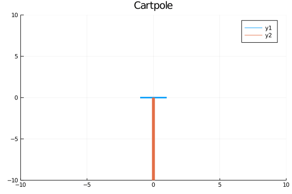
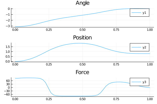
gr()x, dx, theta, dtheta, force = dataanim = Animation()plt=plot(tsteps,[modpi.(theta.+.01),x,force],title=["Angle" "Position" "Force"],layout=(3,1))display(plt)savefig(plt,"cartpole_data.png")for (x, theta) in zip(x, theta)cart = [x - 1 x + 1; 0 0]    pole = [x x + 10*sin(theta); 0 10*cos(theta)]    plt = plot(        cart[1, :],        cart[2, :],        xlim = (-10, 10),        ylim = (-10, 10),        title = "Cartpole",        linewidth = 3,    )    plot!(plt, pole[1, :], pole[2, :], linewidth = 6)frame(anim)endgif(anim, "cartpole_animation.gif", fps = 10)

结果 (Results)

Training to a decent solution takes less than a minute! The controller (agent) neural network first accelerates the cart rapidly to swing the pole. It lets the pole clear the horizon on its angular momentum and then accelerates the cart in the opposite direction to continue the pole’s ascent. Finally, it does a small correction for a standstill at the upright position. Perfecto! We didn’t tell it how to move. It learned on its own!

培训一个体面的解决方案只需不到一分钟！ 控制器(代理)神经网络首先使推车快速加速以摆动杆。 它可以使杆清除其角动量上的地平线，然后沿相反方向加速推车以继续杆的上升。 最后，它会为在直立位置的静止状态做一些小的校正。 完美！ 我们没有告诉它如何移动。 它是自己学习的！

Beauty of the method lies in its versatility. If the objectives and constraints change, we can change the loss function accordingly. If there’s friction and we wish to minimize the energy loss, we simply add a friction term to the model and tag on a frictional power integral in the loss function.

该方法的优点在于其多功能性。 如果目标和约束条件发生变化，我们可以相应地更改损失函数。 如果存在摩擦并且希望将能量损失降至最低，则只需在模型中添加一个摩擦项，然后在损失函数中标记一个摩擦力积分即可。

To illustrate, suppose our mechanical engineer says the motor can’t generate the 60 N peak force demanded by the controller. Actuator limits are common in real life. Motors, fans, pumps all have finite capacity. To reduce the force, we add a max force penalty to the loss function. Also, we increase the time allotted to 10s.

为了说明这一点，假设我们的机械工程师说电动机不能产生控制器要求的60 N峰值力。 执行器极限在现实生活中很常见。 电动机，风扇，泵都具有有限的容量。 为了减小力，我们在损失函数中增加了最大力损失。 另外，我们将分配的时间增加到10s。

tspan = (0.0, 10.0)...loss = sum(theta .^ 2) / N + 4theta[end]^2 + dx[end]^2 + .1sum(x .^ 2) / N + .001maximum(force.^2)

Guess what happens upon training?

猜猜训练后会发生什么？

Ingenious! The AI taps into the natural system resonance like a child on a swing. It periodically accelerates and decelerates to couple energy into the pole, which reduces the peak force required by 10x!

巧妙！ AI像Swing上的孩子一样，进入自然系统的共振。 它会周期性地加速和减速以将能量耦合到磁极中，从而将所需的峰值力降低了10倍！

注意事项 (Caveats)

Neural ODEs can be prone to local minima or underfitting. This isn’t due to the neural network but rather the natural minima of the system. For example, depending on the loss function, the cart can end up not moving. In the language of the calculus of variations, any perturbation to the starting trajectory may in fact increase the loss. In such cases, one needs to adjust the loss function, perhaps penalizing the system for staying still at the beginning. See https://diffeqflux.sciml.ai/dev/examples/local_minima/

神经ODE可能容易出现局部最小值或拟合不足。 这不是由于神经网络，而是由于系统的自然最小值。 例如，根据损失功能，推车可能最终不动。 用变化演算的语言来说，对起始轨迹的任何干扰实际上都可能增加损失。 在这种情况下，需要调整损失函数，也许会损害系统起步时的静止状态。 参见https://diffeqflux.sciml.ai/dev/examples/local_minima/

讨论区 (Discussion)

The astute data scientist may recognize this as the policy gradient method to reinforcement learning. It’s also equivalent to state feedback using neural networks as researched in control theory. These are considered fairly advanced methods, but our neural ODE formulation dramatically simplifies their implementation.

精明的数据科学家可能将其视为加强学习的策略梯度方法。 这也等效于控制理论中研究的使用神经网络的状态反馈。 这些方法被认为是相当先进的方法，但是我们的神经ODE公式极大地简化了它们的实现。

First, neural ODE is a continuum model that requires no time discretization or interpolation of the dynamics. The ODE solver is instructed to sample at whatever time points necessary to compute the loss.

首先，神经ODE是一个连续模型，不需要时间离散化或动力学插值。 指示ODE求解器在计算损失所需的任何时间点进行采样。

Second, the Julia implementation of neural ODE uses automatic differentiation (AD) to efficiently compute gradients for arbitrary functions! This is the magic behind the 1-line “train” method. Recall back propagation in deep learning is simply the chain rule. Tensorflow and Pytorch does this on graphs of predefined neural network building blocks in their libraries, whereas Julia’s Flux (and Zygote underneath) does this for arbitrary functions written in Julia! Not only did it back propagate through our controller network, it did the same with the ODE solver itself. All we did was defining the ODE and loss function.

其次，神经ODE的Julia实现使用自动微分(AD)来有效地计算任意函数的梯度！ 这就是1行“火车”方法背后的魔力。 回顾深度学习中的回传传播只是链式规则。 Tensorflow和Pytorch在其库中预定义的神经网络构建图上执行此操作，而Julia的Flux(及其下的Zygote)对执行Julia编写的任意函数执行此操作！ 它不仅通过我们的控制器网络传播回来，而且与ODE求解器本身一样。 我们所做的只是定义ODE和损失函数。

Third, we can make the system simulation data driven. There, we can replace the physics (or part thereof) with a system dynamics neural network. We train it on observation data, such as sensors time series from a vehicle or industrial process. Then, we stick in the controller neural network to compute optimal control.

第三，我们可以使系统仿真数据驱动。 在那里，我们可以用系统动力学神经网络代替物理学(或其一部分)。 我们根据观察数据(例如来自车辆或工业过程的传感器时间序列)对其进行训练。 然后，我们使用控制器神经网络来计算最佳控制。

致谢 (Acknowledgment)

Thanks to the open source Julia community: Chris Rackauckas for DiffEqFlux, Mike Innes for Zygote, and many others..

感谢开源的Julia社区：DiffEqFlux的Chris Rackauckas，Zygote的Mike Innes以及其他许多人。

参考和教程 (References & Tutorials)

Neural Ordinary Differential Equations. https://arxiv.org/abs/1806.07366* Original neural ODE paper

神经常微分方程。 https://arxiv.org/abs/1806.07366 *原始神经ODE论文

Neural Ordinary Differential Equations with sciml_train. https://diffeqflux.sciml.ai/dev/examples/neural_ode_sciml/* Julia code for variety of neural ODE applications

具有sciml_train的神经常微分方程。 https://diffeqflux.sciml.ai/dev/examples/neural_ode_sciml/ *用于各种神经ODE应用程序的Julia代码

A Differentiable Programming System to Bridge Machine Learning and Scientific Computing. https://arxiv.org/abs/1907.07587* Applications of differentiable programming

桥接机器学习和科学计算的可区分编程系统。 https://arxiv.org/abs/1907.07587 *可微编程的应用

最后… (Finally…)

I’d love to help if you have a question, idea or problem. Leave a message :)

如果您有任何疑问，想法或问题，我很乐意提供帮助。 留言 ：)