转载自：https://towardsdatascience.com/recognizing-traffic-signs-with-over-98-accuracy-using-deep-learning-86737aedc2ab

Recognising Traffic Signs With 98% Accuracy Using Deep Learning

Eddie ForsonFollow

Aug 23, 2017

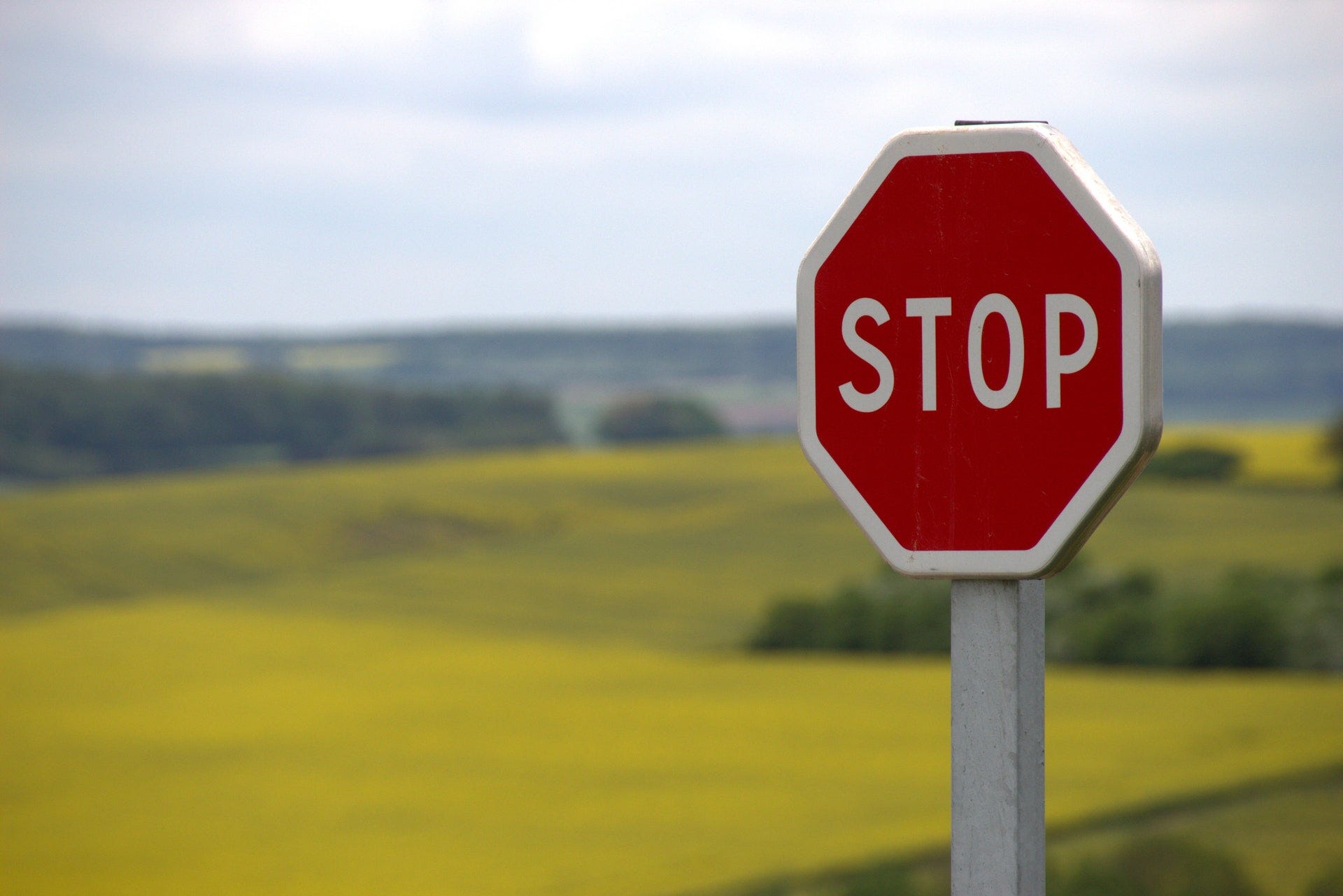
Stop Sign

This is project 2 of Term 1 of the Udacity Self-Driving Car Engineer Nanodegree. You can find all code related to this project on github. You can also read my post on project 1: Detecting Lane Lines Using Computer Vision by simply clicking on the link.

Traffic signs are an integral part of our road infrastructure. They provide critical information, sometimes compelling recommendations, for road users, which in turn requires them to adjust their driving behaviour to make sure they adhere with whatever road regulation currently enforced. Without such useful signs, we would most likely be faced with more accidents, as drivers would not be given critical feedback on how fast they could safely go, or informed about road works, sharp turn, or school crossings ahead. In our modern age, around 1.3M people die on roads each year. This number would be much higher without our road signs.
Naturally, autonomous vehicles must also abide by road legislation and therefore recognize and understand traffic signs.

Traditionally, standard computer vision methods were employed to detect and classify traffic signs, but these required considerable and time-consuming manual work to handcraft important features in images. Instead, by applying deep learning to this problem, we create a model that reliably classifies traffic signs, learning to identify the most appropriate features for this problem by itself. In this post, I show how we can create a deep learning architecture that can identify traffic signs with close to 98% accuracy on the test set.

Project Setup

The dataset is plit into training, test and validation sets, with the following characteristics:

Images are 32 (width) x 32 (height) x 3 (RGB color channels)
Training set is composed of 34799 images
Validation set is composed of 4410 images
Test set is composed of 12630 images
There are 43 classes (e.g. Speed Limit 20km/h, No entry, Bumpy road, etc.)

Moreover, we will be using Python 3.5 with Tensorflow to write our code.

Images And Distribution

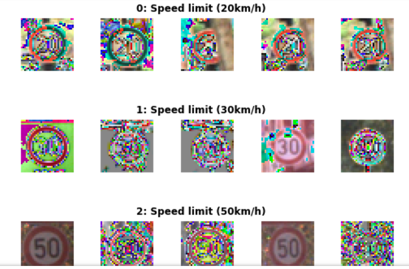
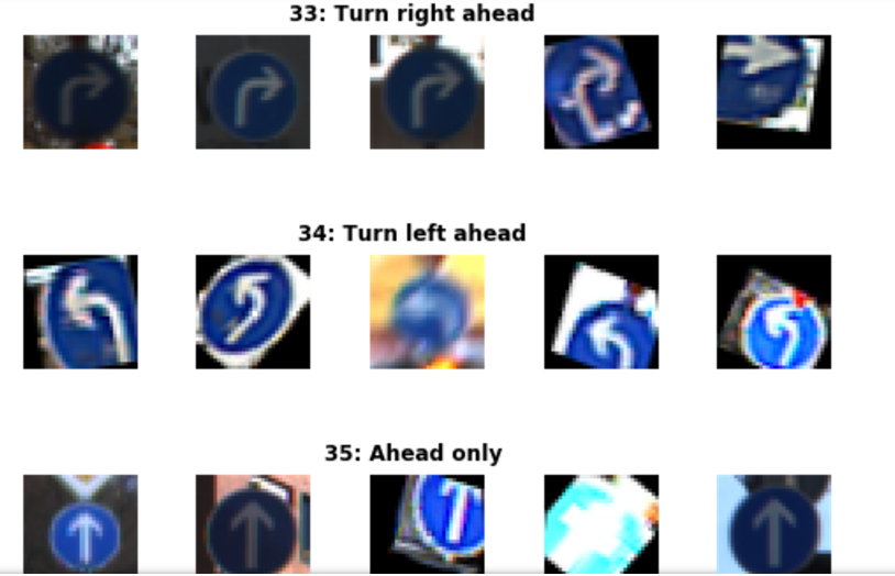
You can see below a sample of the images from the dataset, with labels displayed above the row of corresponding images. Some of them are quite dark so we will look to improve contrast a bit later.

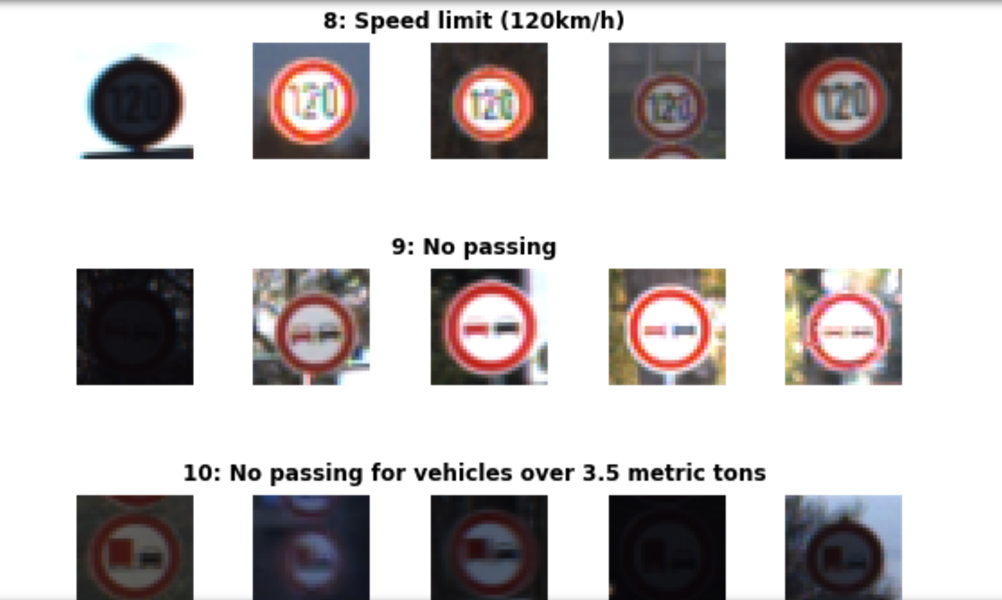
Sample of Training Set Images With Labels Above

There is also a significant imbalance across classes in the training set, as shown in the histogram below. Some classes have less than 200 images, while others have over 2000. This means that our model could be biased towards over-represented classes, especially when it is unsure in its predictions. We will see later how we can mitigate this discrepancy using data augmentation.

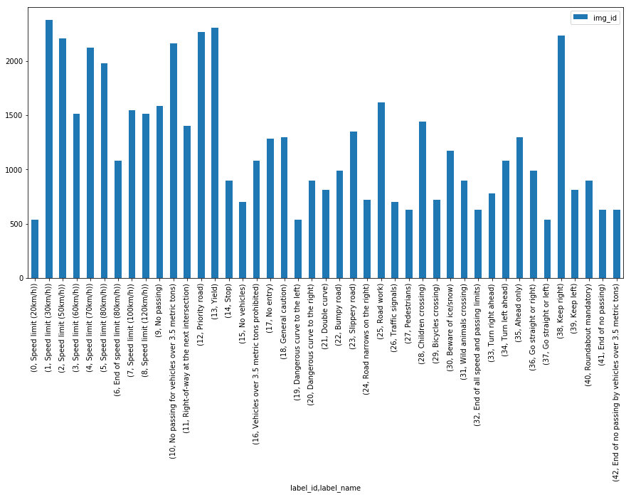
Distribution of images in training set — not quite balanced

Pre-Processing Steps

We initially apply two pre-processing steps to our images:

Grayscale
We convert our 3 channel image to a single grayscale image (we do the same thing in project 1 — Lane Line Detection — you can read my blog post about it HERE).

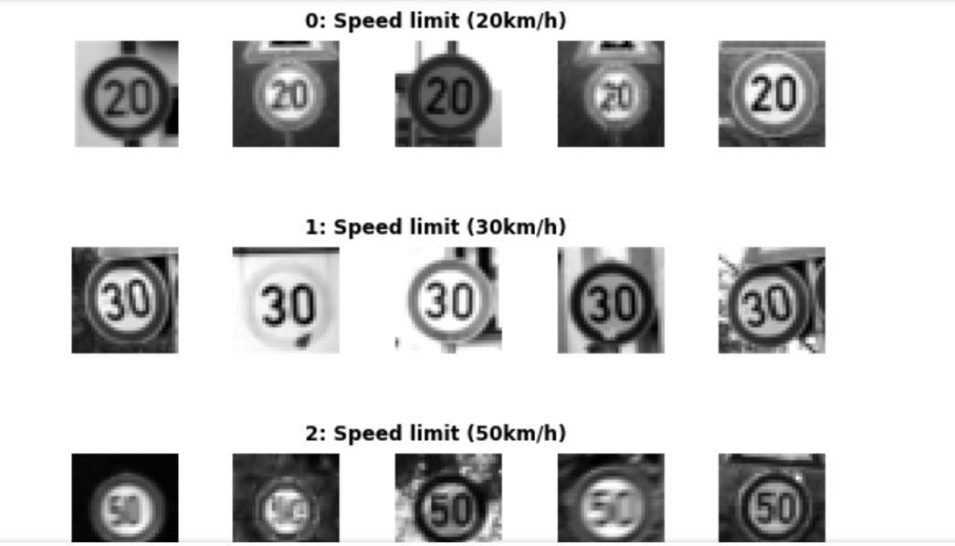
Sample Of Grayscale Training Set Images, with labels above

Image Normalisation
We center the distribution of the image dataset by subtracting each image by the dataset mean and divide by its standard deviation. This helps our model treating images uniformly. The resulting images look as follows:

Normalised images — we can see how “noise” is distributed

Model Architecture

The architecture proposed is inspired from Yann Le Cun’s paper on classification of traffic signs. We added a few tweaks and created a modular codebase which allows us to try out different filter sizes, depth, and number of convolution layers, as well as the dimensions of fully connected layers. In homage to Le Cun, and with a touch of cheekiness, we called such network EdLeNet :).

We mainly tried 5x5 and 3x3 filter (aka kernel) sizes, and start with depth of 32 for our first convolutional layer. EdLeNet’s 3x3 architecture is shown below:

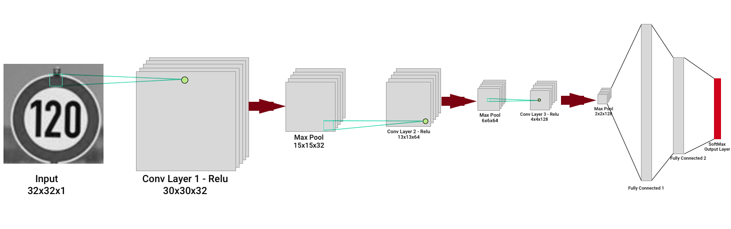
EdLeNet 3x3 Architecture

The network is composed of 3 convolutional layers — kernel size is 3x3, with depth doubling at next layer — using ReLU as the activation function, each followed by a 2x2 max pooling operation. The last 3 layers are fully connected, with the final layer producing 43 results (the total number of possible labels) computed using the SoftMax activation function. The network is trained using mini-batch stochastic gradient descent with the Adamoptimizer. We build a highly modular coding infrastructure that enables us to dynamically create our models like in the following snippets:

mc_3x3 = ModelConfig(EdLeNet, "EdLeNet_Norm_Grayscale_3x3_Dropout_0.50", [32, 32, 1], [3, 32, 3], [120, 84], n_classes, [0.75, 0.5])
mc_5x5 = ModelConfig(EdLeNet, "EdLeNet_Norm_Grayscale_5x5_Dropout_0.50", [32, 32, 1], [5, 32, 2], [120, 84], n_classes, [0.75, 0.5])me_g_norm_drpt_0_50_3x3 = ModelExecutor(mc_3x3)
me_g_norm_drpt_0_50_5x5 = ModelExecutor(mc_5x5)

The ModelConfig contains information about the model such as:

The model function (e.g. EdLeNet)
the model name
input format (e.g. [32, 32, 1] for grayscale),
convolutional layers config [filter size, start depth, number of layers],
fully connected layers dimensions (e.g. [120, 84])
number of classes
dropout keep percentage values [p-conv, p-fc]

The ModelExecutor is reponsible for training, evaluating, predicting, and producing visualizations of our activation maps.

To better isolate our models and make sure they do not all exist under the same Tensorflow graph, we use the following useful construct:

self.graph = tf.Graph()
with self.graph.as_default() as g:with g.name_scope( self.model_config.name ) as scope:...with tf.Session(graph = self.graph) as sess:

This way, we create separate graphs for every model, making sure there is no mixing of our variables, placeholders etc. It’s saved me a lot of headaches.

We actually started with a convolutional depth of 16, but obtained better results with 32 so settled on this value. We also compared color vs grayscale, standard and normalised images, and saw that grayscale tended to outperform color. Unfortunately, we barely scratched 93% test set accuracy on 3x3 or 5x5 models, not consistently reaching this milestone. Moreover, we observed some erratic loss behaviour on the validation set after a given number of epochs, which actually meant our model was overfitting on the training set and not generalising. You can see below some of our metric graphs for different model configurations.

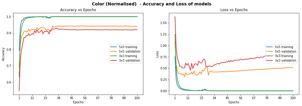
Models Performance on Color Normalised Images

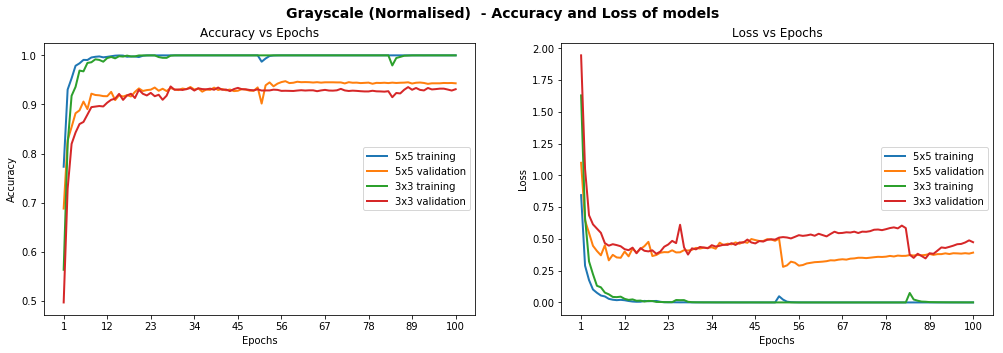
Models Performance On Grayscale Normalised Images

Dropout

In order to improve the model reliability, we turned to dropout, which is a form of regularisation where weights are kept with a probability p: the unkept weights are thus “dropped”. This prevents the model from overfitting. Dropout was introduced by Geoffrey Hinton, a pioneer in the deep learning space. His group’s paper on this topic is a must read to better understand the motivations behind the authors. There’s also a fascinating parallel with biology and evolution.
In the paper, the authors apply varying degrees of dropout, depending on the type of layer. I therefore decided to adopt a similar approach, defining two levels of dropout, one for convolutional layers, the other for fully connected layers:

p-conv: probability of keeping weight in convolutional layer
p-fc: probability of keeping weight in fully connected layer

Moreover, the authors gradually adopted more aggressive (i.e. lower) values of dropout as they go deeper in the network. Therefore I also decided:

p-conv >= p-fc

that is, we will keep weights with a greater than or equal probability in the convolutional than fully connected layers. The way to reason about this is that we treat the network as a funnel and therefore want to gradually tighten it as we move deeper into the layers: we don’t want to discard too much information at the start as some of it would be extremely valuable. Besides, as we apply MaxPooling in the convolutional layers, we are already losing a bit of information.

We tried different paratemers but ultimately settled on p-conv=0.75 and p-fc=0.5, which enabled us to achieve a test set accuracy of 97.55% on normalised grayscale images with the 3x3 model. Interestingly, we achieved over 98.3% accuracy on the validation set:

Training EdLeNet_Norm_Grayscale_3x3_Dropout_0.50 [epochs=100, batch_size=512]...[1]    total=5.222s | train: time=3.139s, loss=3.4993, acc=0.1047 | val: time=2.083s, loss=3.5613, acc=0.1007
[10]    total=5.190s | train: time=3.122s, loss=0.2589, acc=0.9360 | val: time=2.067s, loss=0.3260, acc=0.8973
...
[90]    total=5.193s | train: time=3.120s, loss=0.0006, acc=0.9999 | val: time=2.074s, loss=0.0747, acc=0.9841
[100]   total=5.191s | train: time=3.123s, loss=0.0004, acc=1.0000 | val: time=2.068s, loss=0.0849, acc=0.9832
Model ./models/EdLeNet_Norm_Grayscale_3x3_Dropout_0.50.chkpt saved
[EdLeNet_Norm_Grayscale_3x3_Dropout_0.50 - Test Set]    time=0.686s, loss=0.1119, acc=0.9755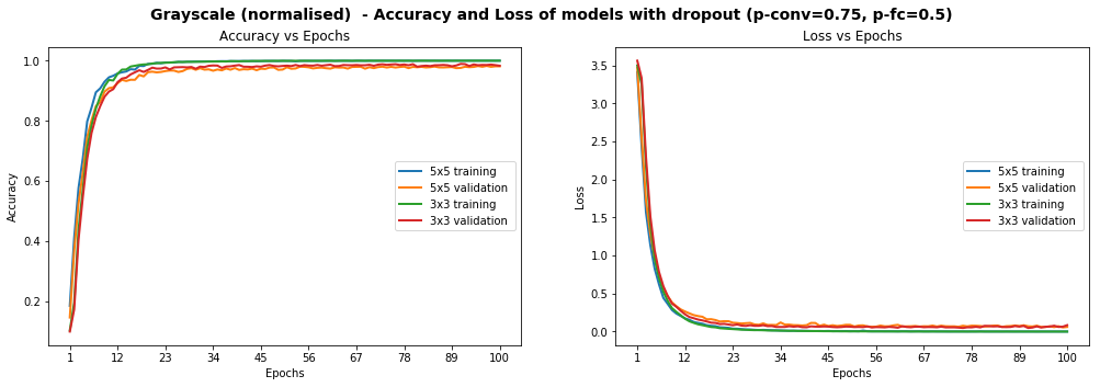

Models Performance on Grayscale Normalised Images, After The Introduction Of Dropout

The graphs above show that the model is smooth, unlike some of the graphs higher up. We have already achieved the objective of scoring over 93% accuracy on the test set, but can we do better? Remember that some of the images were blurry and the distribution of images per class was very uneven. We explore below additional techniques we used to tackle each point.

Histogram Equalization

Histogram Equalization is a computer vision technique used to increase the contrast in images. As some of our images suffer from low contrast (blurry, dark), we will improve visibility by applying OpenCV’s Contrast Limiting Adaptive Histogram Equalization (aka CLAHE) function.

We once again try various configurations, and find the best results, with test accuracy of 97.75%, on the 3x3 model using the following dropout values: p-conv=0.6, p-fc=0.5 .

Training EdLeNet_Grayscale_CLAHE_Norm_Take-2_3x3_Dropout_0.50 [epochs=500, batch_size=512]...

[1]  total=5.194s | train: time=3.137s, loss=3.6254, acc=0.0662 | val: time=2.058s, loss=3.6405, acc=0.0655
[10]    total=5.155s | train: time=3.115s, loss=0.8645, acc=0.7121 | val: time=2.040s, loss=0.9159, acc=0.6819
...
[480]   total=5.149s | train: time=3.106s, loss=0.0009, acc=0.9998 | val: time=2.042s, loss=0.0355, acc=0.9884
[490]   total=5.148s | train: time=3.106s, loss=0.0007, acc=0.9998 | val: time=2.042s, loss=0.0390, acc=0.9884
[500]   total=5.148s | train: time=3.104s, loss=0.0006, acc=0.9999 | val: time=2.044s, loss=0.0420, acc=0.9862
Model ./models/EdLeNet_Grayscale_CLAHE_Norm_Take-2_3x3_Dropout_0.50.chkpt saved
[EdLeNet_Grayscale_CLAHE_Norm_Take-2_3x3_Dropout_0.50 - Test Set]   time=0.675s, loss=0.0890, acc=0.9775

We show below graphs of previous runs where we tested the 5x5 model as well, over 220 epochs. We can see a much smoother curve here, reinforcing our intuition that the model we have is more stable.

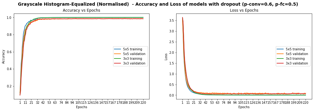
Models Performance On Grayscale Equalized Images, With Dropout

We identified 269 images that are model could not identify correctly. We display 10 of them below, chosen randomly, to conjecture why the model was wrong.

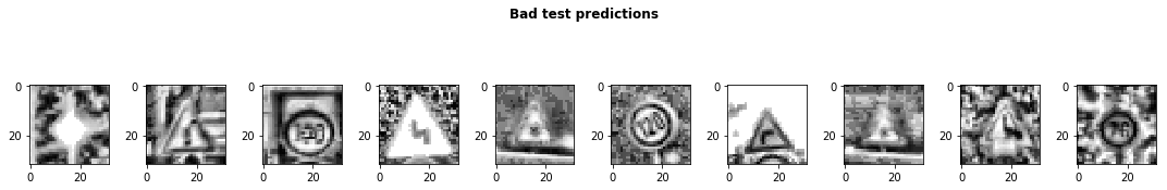
Sample of 10 images where our model got the predictions wrong

Some of the images are very blurry, despite our histogram equalization, while others seem distorted. We probably don’t have enough examples of such images in our test set for our model’s predictions to improve. Additionally, while 97.75% test accuracy is very good, we still one more ace up our sleeve: data augmentation.

Data Augmentation

We observed earlier that the data presented glaring imbalance across the 43 classes. Yet it does not seem to be a crippling problem as we are able to reach very high accuracy despite the class imbalance. We also noticed that some images in the test set are distorted. We are therefore going to use data augmentation techniques in an attempt to:

Extend dataset and provide additional pictures in different lighting settings and orientations
Improve model’s ability to become more generic
Improve test and validation accuracy, especially on distorted images

We use a nifty library called imgaug to create our augmentations. We mainly apply affine transformations to augment the images. Our code looks as follows:

def augment_imgs(imgs, p):"""Performs a set of augmentations with with a probability p"""augs =  iaa.SomeOf((2, 4),[iaa.Crop(px=(0, 4)), # crop images from each side by 0 to 4px (randomly chosen)iaa.Affine(scale={"x": (0.8, 1.2), "y": (0.8, 1.2)}),iaa.Affine(translate_percent={"x": (-0.2, 0.2), "y": (-0.2, 0.2)}),iaa.Affine(rotate=(-45, 45)), # rotate by -45 to +45 degrees)iaa.Affine(shear=(-10, 10)) # shear by -10 to +10 degrees])

    seq = iaa.Sequential([iaa.Sometimes(p, augs)])return seq.augment_images(imgs)

While the class imbalance probably causes some bias in the model, we have decided not to address it at this stage as it would cause our dataset to swell significantly and lengthen our training time (we don’t have a lot of time to spend on training at this stage). Instead, we decided to augment each class by 10%. Our new dataset looks as follows.

Sample Of Augmented Images

The distribution of images does not change significantly of course, but we do apply grayscale, histogram equalization and normalisation pre-processing steps to our images. We train for 2000 epochs with dropout (p-conv=0.6, p-fc=0.5) and achieve 97.86% accuracy on the test set:

[EdLeNet] Building neural network [conv layers=3, conv filter size=3, conv start depth=32, fc layers=2]
Training EdLeNet_Augs_Grayscale_CLAHE_Norm_Take4_Bis_3x3_Dropout_0.50 [epochs=2000, batch_size=512]...[1] total=5.824s | train: time=3.594s, loss=3.6283, acc=0.0797 | val: time=2.231s, loss=3.6463, acc=0.0687
...
[1970]  total=5.627s | train: time=3.408s, loss=0.0525, acc=0.9870 | val: time=2.219s, loss=0.0315, acc=0.9914
[1980]  total=5.627s | train: time=3.409s, loss=0.0530, acc=0.9862 | val: time=2.218s, loss=0.0309, acc=0.9902
[1990]  total=5.628s | train: time=3.412s, loss=0.0521, acc=0.9869 | val: time=2.216s, loss=0.0302, acc=0.9900
[2000]  total=5.632s | train: time=3.415s, loss=0.0521, acc=0.9869 | val: time=2.217s, loss=0.0311, acc=0.9902
Model ./models/EdLeNet_Augs_Grayscale_CLAHE_Norm_Take4_Bis_3x3_Dropout_0.50.chkpt saved

[EdLeNet_Augs_Grayscale_CLAHE_Norm_Take4_Bis_3x3_Dropout_0.50 - Test Set]  time=0.678s, loss=0.0842, acc=0.9786

This is our best performance so far!!!

Neural Network Celebration

But… if you look at the loss metric on the training set, you can see that at 0.0521, we most likely still have some wiggle room. We are planning to train for more epochs and will report on our new results in the future.

Testing On New Images

We decided to test our model on new images as well, to make sure that it’s indeed generalised to more than the traffic signs in our original dataset. We therefore downloaded five new images and submitted them to our model for predictions.

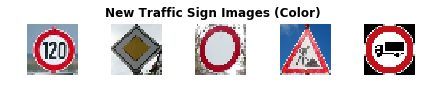
Download 5 new traffic signs — color

The ground truth for the images is as follows:

['Speed limit (120km/h)','Priority road','No vehicles','Road work','Vehicles over 3.5 metric tons prohibited']

The Images were chosen because of the following:

They represent different traffic signs that we currently classify
They vary in shape and color
They are under different lighting conditions (the 4th one has sunlight reflection)
They are under different orientations (the 3rd one is slanted)
They have different background
The last image is actually a design, not a real picture, and we wanted to test the model against it
Some of them are in under-represented classes

The first step we took was to apply the same CLAHE to those new images, resulting in the following:

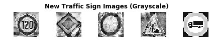
Download 5 new traffic signs — grayscale CLAHE

We achieve perfect accuracy of 100% on the new images. On the original test set, we achieved 97.86% accuracy. We could explore blurring/distorting our new images or modifying contrast to see how the model handles those changes in the future.

new_img_grayscale_norm_pred_acc = np.sum(new_img_lbs == preds) / len(preds)
print("[Grayscale Normalised] Predictional accuracy on new images: {0}%".format(new_img_grayscale_norm_pred_acc * 100))
...
[Grayscale Normalised] Predictional accuracy on new images: 100.0%

We also show the top 5 SoftMax probabilities computed for each image, with the green bar showing the ground truth. We can clearly see that our model is quite confident in its predictions. In the worst case (last image), the 2nd most likely prediction has a probability of around 0.1% . In fact our model struggles most on the last image, which I believe is actually a design and not even a real picture. Overall, we have developed a strong model!

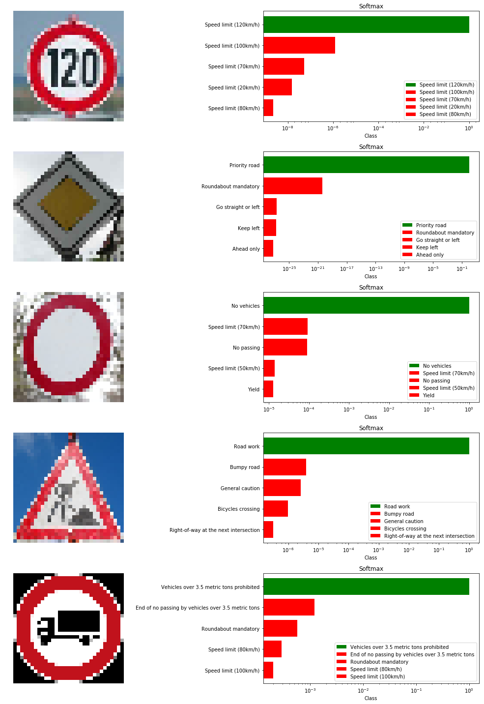
Visualizations of The Model’s Top 5 Predictions

Visualizing Our Activation Maps

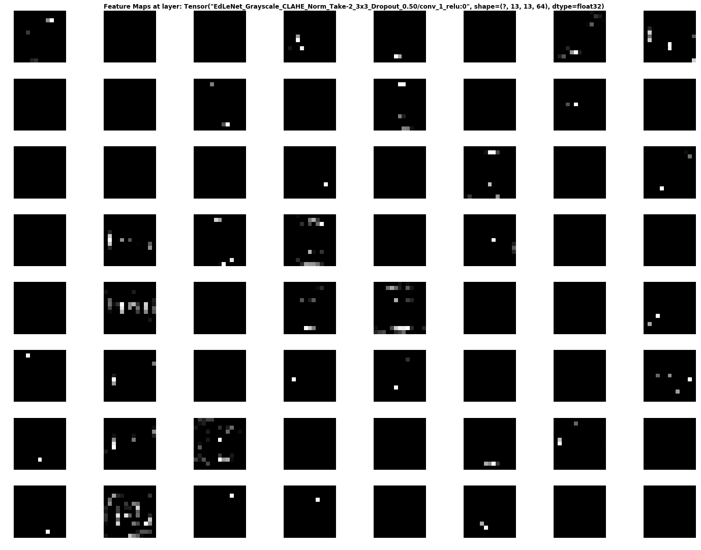
We show below the results produced by each convolutional layer (before max pooling), resulting in 3 activation maps.

Layer 1

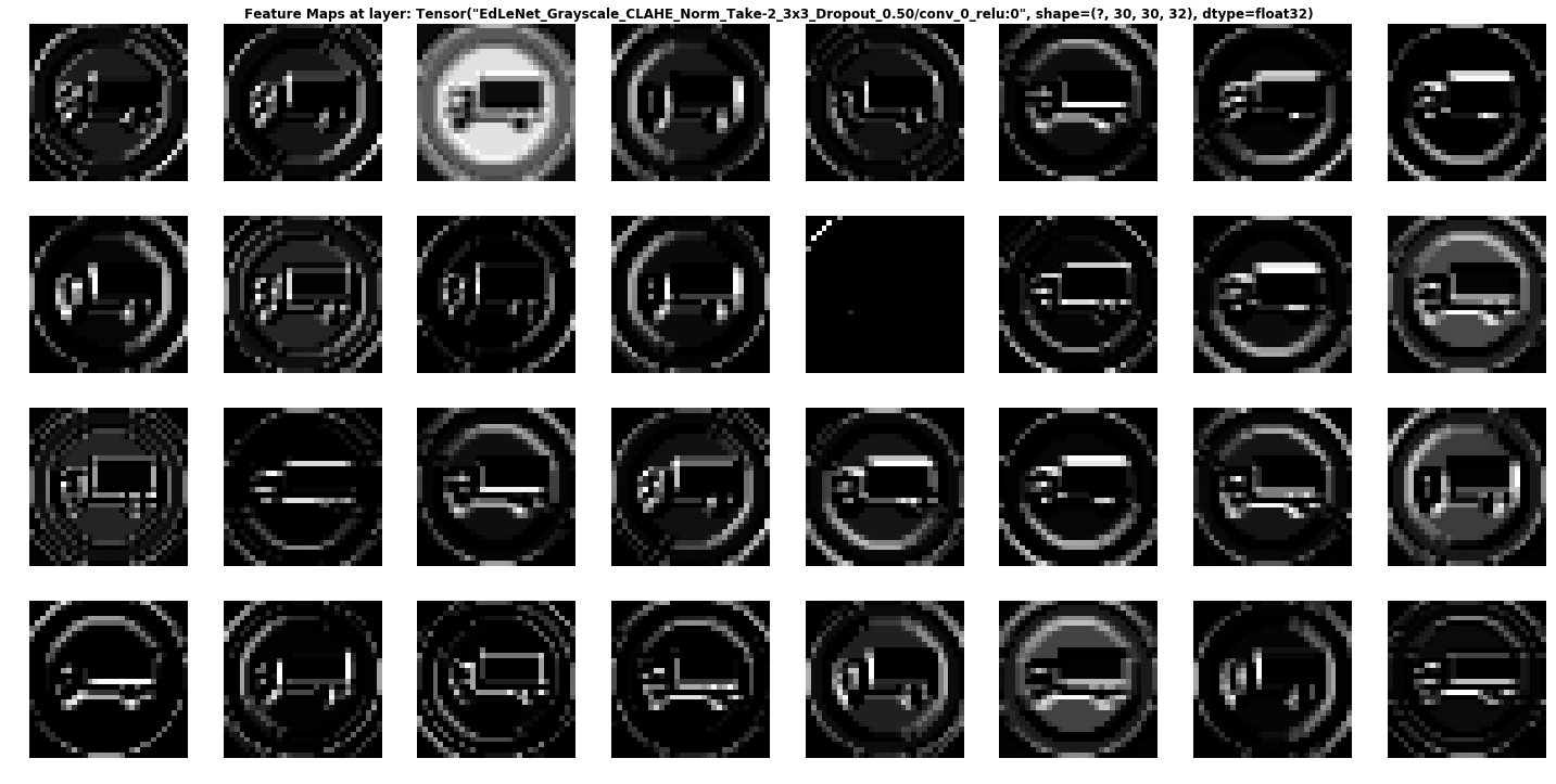
We can see that the network is focusing a lot on the edges of the circle and somehow on the truck. The background is mostly ignored.

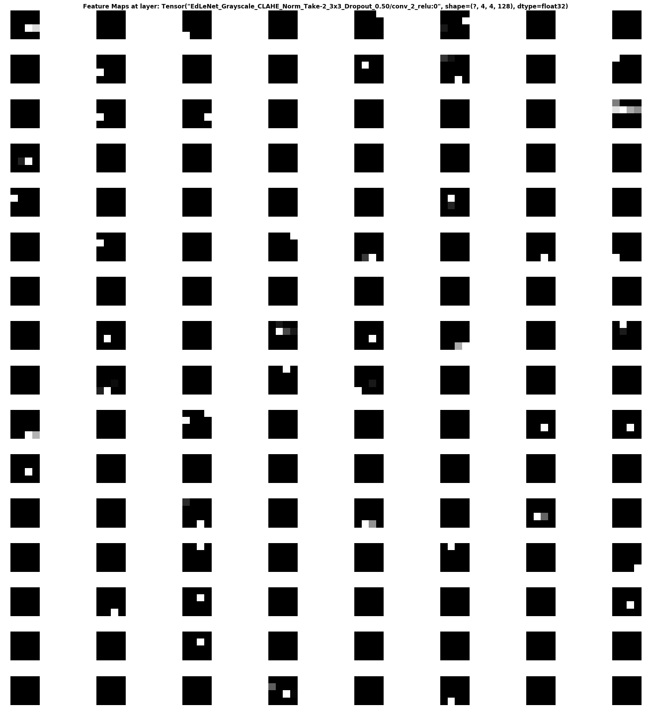
Layer 2

Activation Map Of Second Convolutional Layer

It is rather hard to determine what the network is focusing on in layer 2, but it seems to “activate” around the edges of the circle and in the middle, where the truck appears.

Layer 3

This activation map is also hard to decipher… But it seems the network reacts to stimuli on the edges and in the middle once again.

Conclusion

We covered how deep learning can be used to classify traffic signs with high accuracy, employing a variety of pre-processing and regularization techniques (e.g. dropout), and trying different model architectures. We built highly configurable code and developed a flexible way of evaluating multiple architectures. Our model reached close to close to 98% accuracy on the test set, achieving 99% on the validation set.

Personally, I thoroughly enjoyed this project and gained practical experience using Tensorflow, matplotlib and investigating artificial neural network architectures. Moreover, I delved into some seminal papers in this field, which reinforced my understanding and more importantly refined my intuition about deep learning.

In the future, I believe higher accuracy can be achieved by applying further regularization techniques such as batch normalization and also by adopting more modern architectures such as GoogLeNet’s Inception Module, ResNet, or Xception.

I hope you enjoyed reading this post. Feel free to leave comments and claps :). You also can follow me on Twitter or Medium for more articles on my “AI Journey” . Keep learning and building!

Recognising Traffic Signs相关推荐

CARLA 笔记（06）— Types of actors （Sensors、Spectator、Traffic signs and lights、Vehicles、Walkers）
1. Sensors 此示例生成一个摄像头传感器,将其附加到车辆上,并告诉摄像头将生成的图像保存到磁盘. camera_bp = blueprint_library.find('sensor.came ...
准确率98%的深度学习交通标志识别是如何做到的？
交通标志是道路基础设施的重要组成部分,它们为道路使用者提供了一些关键信息,并要求驾驶员及时调整驾驶行为,以确保遵守道路安全规定.如果没有交通标志,可能会发生更多的事故,因为司机无法获知最高安全速度是多 ...
全新中国交通标志检测数据集2021—CCTSDB 2021: A More Comprehensive Traffic SignDetection Benchmark（全新分类-多算法测评）
CCTSDB 2021 重磅发布! 全新数据集!全新分类!多种算法测评! 欢迎大家使用! 数据集发布网址:GitHub - csust7zhangjm/CCTSDB2021 论文原文:HCIS | A ...
SLAM综述阅读笔记二：Simultaneous Localization and Mapping: A Survey of Current Trends in Autonomous（2017）
转自[第八篇 SLAM:自动驾驶当前趋势综述 - 知乎] 说明该总结主要是针对自动驾驶 <Simultaneous Localization And Mapping: A Survey of C ...
Cybersecurity Challenges In The Uptake Of Artifitial Intelligence in Autonomous Driving [1]
"Cybersecurity Challenges In The Uptake Of Artifitial Intelligence in Autonomous Driving"是 ...
计算机视觉数据集大全 - Part2
转载自http://homepages.inf.ed.ac.uk/rbf/CVonline/Imagedbase.htm Index by Topic Action Databases Agricul ...
Mobileye高级驾驶辅助系统（ADAS）
Mobileye高级驾驶辅助系统(ADAS) Mobileye is the global leader in the development of vision technology for Adv ...
基本机器学习面试问题 ---- Company/Industry Specific/Interest
Machine Learning Interview Questions: Company/Industry Specific These machine learning interview que ...
机器视觉【基础】什么是机器视觉？
前言:本文尝试由繁到简论述机器视觉的定义和发展历程: 1 什么是机器视觉 What is Computer Vision? Computer Vision has a dual goal. From ...

Recognising Traffic Signs