Andrej Karpathy blog

转自：http://karpathy.github.io/2015/05/21/rnn-effectiveness/

Karpathy 关于RNN的博客

The Unreasonable Effectiveness of Recurrent Neural Networks

May 21, 2015

There’s something magical about Recurrent Neural Networks (RNNs). I still remember when I trained my first recurrent network for Image Captioning. Within a few dozen minutes of training my first baby model (with rather arbitrarily-chosen hyperparameters) started to generate very nice looking descriptions of images that were on the edge of making sense. Sometimes the ratio of how simple your model is to the quality of the results you get out of it blows past your expectations, and this was one of those times. What made this result so shocking at the time was that the common wisdom was that RNNs were supposed to be difficult to train (with more experience I’ve in fact reached the opposite conclusion). Fast forward about a year: I’m training RNNs all the time and I’ve witnessed their power and robustness many times, and yet their magical outputs still find ways of amusing me. This post is about sharing some of that magic with you.

We’ll train RNNs to generate text character by character and ponder the question “how is that even possible?”

By the way, together with this post I am also releasing code on Github that allows you to train character-level language models based on multi-layer LSTMs. You give it a large chunk of text and it will learn to generate text like it one character at a time. You can also use it to reproduce my experiments below. But we’re getting ahead of ourselves; What are RNNs anyway?

Recurrent Neural Networks

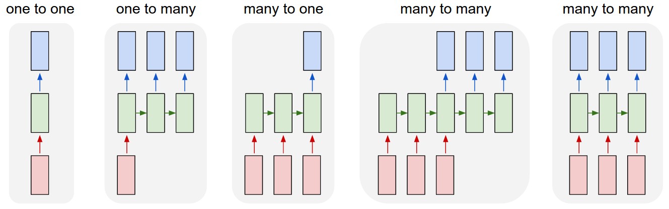
Sequences. Depending on your background you might be wondering: What makes Recurrent Networks so special? A glaring limitation of Vanilla Neural Networks (and also Convolutional Networks) is that their API is too constrained: they accept a fixed-sized vector as input (e.g. an image) and produce a fixed-sized vector as output (e.g. probabilities of different classes). Not only that: These models perform this mapping using a fixed amount of computational steps (e.g. the number of layers in the model). The core reason that recurrent nets are more exciting is that they allow us to operate over sequences of vectors: Sequences in the input, the output, or in the most general case both. A few examples may make this more concrete:

Each rectangle is a vector and arrows represent functions (e.g. matrix multiply). Input vectors are in red, output vectors are in blue and green vectors hold the RNN's state (more on this soon). From left to right: (1) Vanilla mode of processing without RNN, from fixed-sized input to fixed-sized output (e.g. image classification). (2) Sequence output (e.g. image captioning takes an image and outputs a sentence of words). (3) Sequence input (e.g. sentiment analysis where a given sentence is classified as expressing positive or negative sentiment). (4) Sequence input and sequence output (e.g. Machine Translation: an RNN reads a sentence in English and then outputs a sentence in French). (5) Synced sequence input and output (e.g. video classification where we wish to label each frame of the video). Notice that in every case are no pre-specified constraints on the lengths sequences because the recurrent transformation (green) is fixed and can be applied as many times as we like.

As you might expect, the sequence regime of operation is much more powerful compared to fixed networks that are doomed from the get-go by a fixed number of computational steps, and hence also much more appealing for those of us who aspire to build more intelligent systems. Moreover, as we’ll see in a bit, RNNs combine the input vector with their state vector with a fixed (but learned) function to produce a new state vector. This can in programming terms be interpreted as running a fixed program with certain inputs and some internal variables. Viewed this way, RNNs essentially describe programs. In fact, it is known that RNNs are Turing-Complete in the sense that they can to simulate arbitrary programs (with proper weights). But similar to universal approximation theorems for neural nets you shouldn’t read too much into this. In fact, forget I said anything.

If training vanilla neural nets is optimization over functions, training recurrent nets is optimization over programs.

Sequential processing in absence of sequences. You might be thinking that having sequences as inputs or outputs could be relatively rare, but an important point to realize is that even if your inputs/outputs are fixed vectors, it is still possible to use this powerful formalism to process them in a sequential manner. For instance, the figure below shows results from two very nice papers from DeepMind. On the left, an algorithm learns a recurrent network policy that steers its attention around an image; In particular, it learns to read out house numbers from left to right (Ba et al.). On the right, a recurrent network generates images of digits by learning to sequentially add color to a canvas (Gregor et al.):

 

Left: RNN learns to read house numbers. Right: RNN learns to paint house numbers.

The takeaway is that even if your data is not in form of sequences, you can still formulate and train powerful models that learn to process it sequentially. You’re learning stateful programs that process your fixed-sized data.

RNN computation. So how do these things work? At the core, RNNs have a deceptively simple API: They accept an input vector x and give you an output vector y. However, crucially this output vector’s contents are influenced not only by the input you just fed in, but also on the entire history of inputs you’ve fed in in the past. Written as a class, the RNN’s API consists of a single step function:

rnn = RNN()
y = rnn.step(x) # x is an input vector, y is the RNN's output vector 

The RNN class has some internal state that it gets to update every time step is called. In the simplest case this state consists of a single hidden vector h. Here is an implementation of the step function in a Vanilla RNN:

class RNN:# ...def step(self, x): # update the hidden state self.h = np.tanh(np.dot(self.W_hh, self.h) + np.dot(self.W_xh, x)) # compute the output vector y = np.dot(self.W_hy, self.h) return y 

The above specifies the forward pass of a vanilla RNN. This RNN’s parameters are the three matrices W_hh, W_xh, W_hy. The hidden state self.h is initialized with the zero vector. The np.tanh function implements a non-linearity that squashes the activations to the range [-1, 1]. Notice briefly how this works: There are two terms inside of the tanh: one is based on the previous hidden state and one is based on the current input. In numpy np.dot is matrix multiplication. The two intermediates interact with addition, and then get squashed by the tanh into the new state vector. If you’re more comfortable with math notation, we can also write the hidden state update as ht=tanh(Whhht−1+Wxhxt)ht=tanh⁡(Whhht−1+Wxhxt), where tanh is applied elementwise.

We initialize the matrices of the RNN with random numbers and the bulk of work during training goes into finding the matrices that give rise to desirable behavior, as measured with some loss function that expresses your preference to what kinds of outputs y you’d like to see in response to your input sequences x.

Going deep. RNNs are neural networks and everything works monotonically better (if done right) if you put on your deep learning hat and start stacking models up like pancakes. For instance, we can form a 2-layer recurrent network as follows:

y1 = rnn1.step(x) y = rnn2.step(y1) 

In other words we have two separate RNNs: One RNN is receiving the input vectors and the second RNN is receiving the output of the first RNN as its input. Except neither of these RNNs know or care - it’s all just vectors coming in and going out, and some gradients flowing through each module during backpropagation.

Getting fancy. I’d like to briefly mention that in practice most of us use a slightly different formulation than what I presented above called a Long Short-Term Memory (LSTM) network. The LSTM is a particular type of recurrent network that works slightly better in practice, owing to its more powerful update equation and some appealing backpropagation dynamics. I won’t go into details, but everything I’ve said about RNNs stays exactly the same, except the mathematical form for computing the update (the line self.h = ... ) gets a little more complicated. From here on I will use the terms “RNN/LSTM” interchangeably but all experiments in this post use an LSTM.

Character-Level Language Models

Okay, so we have an idea about what RNNs are, why they are super exciting, and how they work. We’ll now ground this in a fun application: We’ll train RNN character-level language models. That is, we’ll give the RNN a huge chunk of text and ask it to model the probability distribution of the next character in the sequence given a sequence of previous characters. This will then allow us to generate new text one character at a time.

As a working example, suppose we only had a vocabulary of four possible letters “helo”, and wanted to train an RNN on the training sequence “hello”. This training sequence is in fact a source of 4 separate training examples: 1. The probability of “e” should be likely given the context of “h”, 2. “l” should be likely in the context of “he”, 3. “l” should also be likely given the context of “hel”, and finally 4. “o” should be likely given the context of “hell”.

Concretely, we will encode each character into a vector using 1-of-k encoding (i.e. all zero except for a single one at the index of the character in the vocabulary), and feed them into the RNN one at a time with the stepfunction. We will then observe a sequence of 4-dimensional output vectors (one dimension per character), which we interpret as the confidence the RNN currently assigns to each character coming next in the sequence. Here’s a diagram:

An example RNN with 4-dimensional input and output layers, and a hidden layer of 3 units (neurons). This diagram shows the activations in the forward pass when the RNN is fed the characters "hell" as input. The output layer contains confidences the RNN assigns for the next character (vocabulary is "h,e,l,o"); We want the green numbers to be high and red numbers to be low.

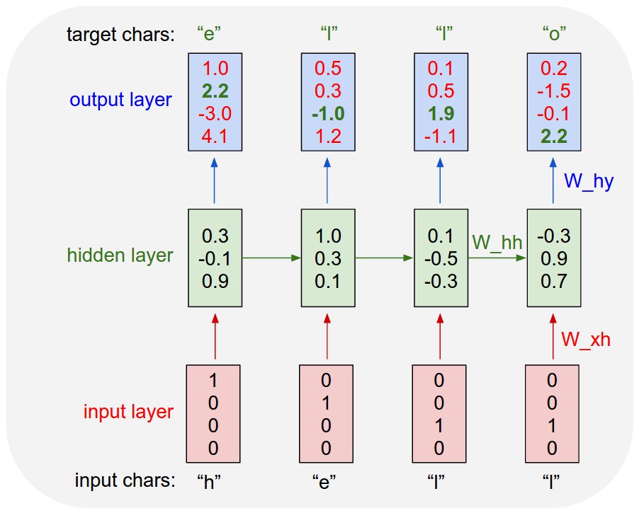
For example, we see that in the first time step when the RNN saw the character “h” it assigned confidence of 1.0 to the next letter being “h”, 2.2 to letter “e”, -3.0 to “l”, and 4.1 to “o”. Since in our training data (the string “hello”) the next correct character is “e”, we would like to increase its confidence (green) and decrease the confidence of all other letters (red). Similarly, we have a desired target character at every one of the 4 time steps that we’d like the network to assign a greater confidence to. Since the RNN consists entirely of differentiable operations we can run the backpropagation algorithm (this is just a recursive application of the chain rule from calculus) to figure out in what direction we should adjust every one of its weights to increase the scores of the correct targets (green bold numbers). We can then perform a parameter update, which nudges every weight a tiny amount in this gradient direction. If we were to feed the same inputs to the RNN after the parameter update we would find that the scores of the correct characters (e.g. “e” in the first time step) would be slightly higher (e.g. 2.3 instead of 2.2), and the scores of incorrect characters would be slightly lower. We then repeat this process over and over many times until the network converges and its predictions are eventually consistent with the training data in that correct characters are always predicted next.

A more technical explanation is that we use the standard Softmax classifier (also commonly referred to as the cross-entropy loss) on every output vector simultaneously. The RNN is trained with mini-batch Stochastic Gradient Descent and I like to use RMSProp or Adam (per-parameter adaptive learning rate methods) to stablilize the updates.

Notice also that the first time the character “l” is input, the target is “l”, but the second time the target is “o”. The RNN therefore cannot rely on the input alone and must use its recurrent connection to keep track of the context to achieve this task.

At test time, we feed a character into the RNN and get a distribution over what characters are likely to come next. We sample from this distribution, and feed it right back in to get the next letter. Repeat this process and you’re sampling text! Lets now train an RNN on different datasets and see what happens.

To further clarify, for educational purposes I also wrote a minimal character-level RNN language model in Python/numpy. It is only about 100 lines long and hopefully it gives a concise, concrete and useful summary of the above if you’re better at reading code than text. We’ll now dive into example results, produced with the much more efficient Lua/Torch codebase.

Fun with RNNs

All 5 example character models below were trained with the code I’m releasing on Github. The input in each case is a single file with some text, and we’re training an RNN to predict the next character in the sequence.

Paul Graham generator

Lets first try a small dataset of English as a sanity check. My favorite fun dataset is the concatenation of Paul Graham’s essays. The basic idea is that there’s a lot of wisdom in these essays, but unfortunately Paul Graham is a relatively slow generator. Wouldn’t it be great if we could sample startup wisdom on demand? That’s where an RNN comes in.

Concatenating all pg essays over the last ~5 years we get approximately 1MB text file, or about 1 million characters (this is considered a very small dataset by the way). Technical: Lets train a 2-layer LSTM with 512 hidden nodes (approx. 3.5 million parameters), and with dropout of 0.5 after each layer. We’ll train with batches of 100 examples and truncated backpropagation through time of length 100 characters. With these settings one batch on a TITAN Z GPU takes about 0.46 seconds (this can be cut in half with 50 character BPTT at negligible cost in performance). Without further ado, lets see a sample from the RNN:

“The surprised in investors weren’t going to raise money. I’m not the company with the time there are all interesting quickly, don’t have to get off the same programmers. There’s a super-angel round fundraising, why do you can do. If you have a different physical investment are become in people who reduced in a startup with the way to argument the acquirer could see them just that you’re also the founders will part of users’ affords that and an alternation to the idea. [2] Don’t work at first member to see the way kids will seem in advance of a bad successful startup. And if you have to act the big company too.”

Okay, clearly the above is unfortunately not going to replace Paul Graham anytime soon, but remember that the RNN had to learn English completely from scratch and with a small dataset (including where you put commas, apostrophes and spaces). I also like that it learns to support its own arguments (e.g. [2], above). Sometimes it says something that offers a glimmer of insight, such as “a company is a meeting to think to investors”. Here’s a link to 50K character sample if you’d like to see more.

Temperature. We can also play with the temperature of the Softmax during sampling. Decreasing the temperature from 1 to some lower number (e.g. 0.5) makes the RNN more confident, but also more conservative in its samples. Conversely, higher temperatures will give more diversity but at cost of more mistakes (e.g. spelling mistakes, etc). In particular, setting temperature very near zero will give the most likely thing that Paul Graham might say:

“is that they were all the same thing that was a startup is that they were all the same thing that was a startup is that they were all the same thing that was a startup is that they were all the same”

looks like we’ve reached an infinite loop about startups.

Shakespeare

It looks like we can learn to spell English words. But how about if there is more structure and style in the data? To examine this I downloaded all the works of Shakespeare and concatenated them into a single (4.4MB) file. We can now afford to train a larger network, in this case lets try a 3-layer RNN with 512 hidden nodes on each layer. After we train the network for a few hours we obtain samples such as:

PANDARUS:
Alas, I think he shall be come approached and the day
When little srain would be attain'd into being never fed,
And who is but a chain and subjects of his death,
I should not sleep.Second Senator:
They are away this miseries, produced upon my soul,
Breaking and strongly should be buried, when I perish
The earth and thoughts of many states.DUKE VINCENTIO:
Well, your wit is in the care of side and that.Second Lord:
They would be ruled after this chamber, and
my fair nues begun out of the fact, to be conveyed,
Whose noble souls I'll have the heart of the wars.Clown:
Come, sir, I will make did behold your worship.VIOLA:
I'll drink it.

Remember, all the RNN knows are characters, so in particular it samples both speaker’s names and the contents. Sometimes we also get relatively extented monologue passages, such as:

VIOLA:
Why, Salisbury must find his flesh and thought
That which I am not aps, not a man and in fire,
To show the reining of the raven and the wars
To grace my hand reproach within, and not a fair are hand,
That Caesar and my goodly father's world;
When I was heaven of presence and our fleets,
We spare with hours, but cut thy council I am great,
Murdered and by thy master's ready there
My power to give thee but so much as hell:
Some service in the noble bondman here,
Would show him to her wine.KING LEAR:
O, if you were a feeble sight, the courtesy of your law,
Your sight and several breath, will wear the gods
With his heads, and my hands are wonder'd at the deeds,
So drop upon your lordship's head, and your opinion
Shall be against your honour.

I can barely recognize these samples from actual Shakespeare :) If you like Shakespeare, you might appreciate this 100,000 character sample. Of course, you can also generate an infinite amount of your own samples at different temperatures with the provided code.

Wikipedia

We saw that the LSTM can learn to spell words and copy general syntactic structures. Lets further increase the difficulty and train on structured markdown. In particular, lets take the Hutter Prize 100MB dataset of raw Wikipedia and train an LSTM. Following Graves et al., I used the first 96MB for training, the rest for validation and ran a few models overnight. We can now sample Wikipedia articles! Below are a few fun excerpts. First, some basic markdown output:

Naturalism and decision for the majority of Arab countries' capitalide was grounded
by the Irish language by [[John Clair]], [[An Imperial Japanese Revolt]], associated
with Guangzham's sovereignty. His generals were the powerful ruler of the Portugal
in the [[Protestant Immineners]], which could be said to be directly in Cantonese
Communication, which followed a ceremony and set inspired prison, training. The
emperor travelled back to [[Antioch, Perth, October 25|21]] to note, the Kingdom
of Costa Rica, unsuccessful fashioned the [[Thrales]], [[Cynth's Dajoard]], known
in western [[Scotland]], near Italy to the conquest of India with the conflict.
Copyright was the succession of independence in the slop of Syrian influence that
was a famous German movement based on a more popular servicious, non-doctrinal
and sexual power post. Many governments recognize the military housing of the
[[Civil Liberalization and Infantry Resolution 265 National Party in Hungary]],
that is sympathetic to be to the [[Punjab Resolution]]
(PJS)[http://www.humah.yahoo.com/guardian.
cfm/7754800786d17551963s89.htm Official economics Adjoint for the Nazism, Montgomery
was swear to advance to the resources for those Socialism's rule,
was starting to signing a major tripad of aid exile.]]

In case you were wondering, the yahoo url above doesn’t actually exist, the model just hallucinated it. Also, note that the model learns to open and close the parenthesis correctly. There’s also quite a lot of structured markdown that the model learns, for example sometimes it creates headings, lists, etc.:

{ { cite journal | id=Cerling Nonforest Department|format=Newlymeslated|none } }
''www.e-complete''.'''See also''': [[List of ethical consent processing]]== See also ==
*[[Iender dome of the ED]]
*[[Anti-autism]]===[[Religion|Religion]]===
*[[French Writings]]
*[[Maria]]
*[[Revelation]]
*[[Mount Agamul]]== External links==
* [http://www.biblegateway.nih.gov/entrepre/ Website of the World Festival. The labour of India-county defeats at the Ripper of California Road.]==External links==
* [http://www.romanology.com/ Constitution of the Netherlands and Hispanic Competition for Bilabial and Commonwealth Industry (Republican Constitution of the Extent of the Netherlands)]

Sometimes the model snaps into a mode of generating random but valid XML:

<page><title>Antichrist</title><id>865</id><revision><id>15900676</id><timestamp>2002-08-03T18:14:12Z</timestamp><contributor><username>Paris</username><id>23</id></contributor><minor /><comment>Automated conversion</comment><text xml:space="preserve">#REDIRECT [[Christianity]]</text></revision>
</page>

The model completely makes up the timestamp, id, and so on. Also, note that it closes the correct tags appropriately and in the correct nested order. Here are 100,000 characters of sampled wikipedia if you’re interested to see more.

Algebraic Geometry (Latex)

The results above suggest that the model is actually quite good at learning complex syntactic structures. Impressed by these results, my labmate (Justin Johnson) and I decided to push even further into structured territories and got a hold of this book on algebraic stacks/geometry. We downloaded the raw Latex source file (a 16MB file) and trained a multilayer LSTM. Amazingly, the resulting sampled Latex almost compiles. We had to step in and fix a few issues manually but then you get plausible looking math, it’s quite astonishing:

Sampled (fake) algebraic geometry. Here's the actual pdf.

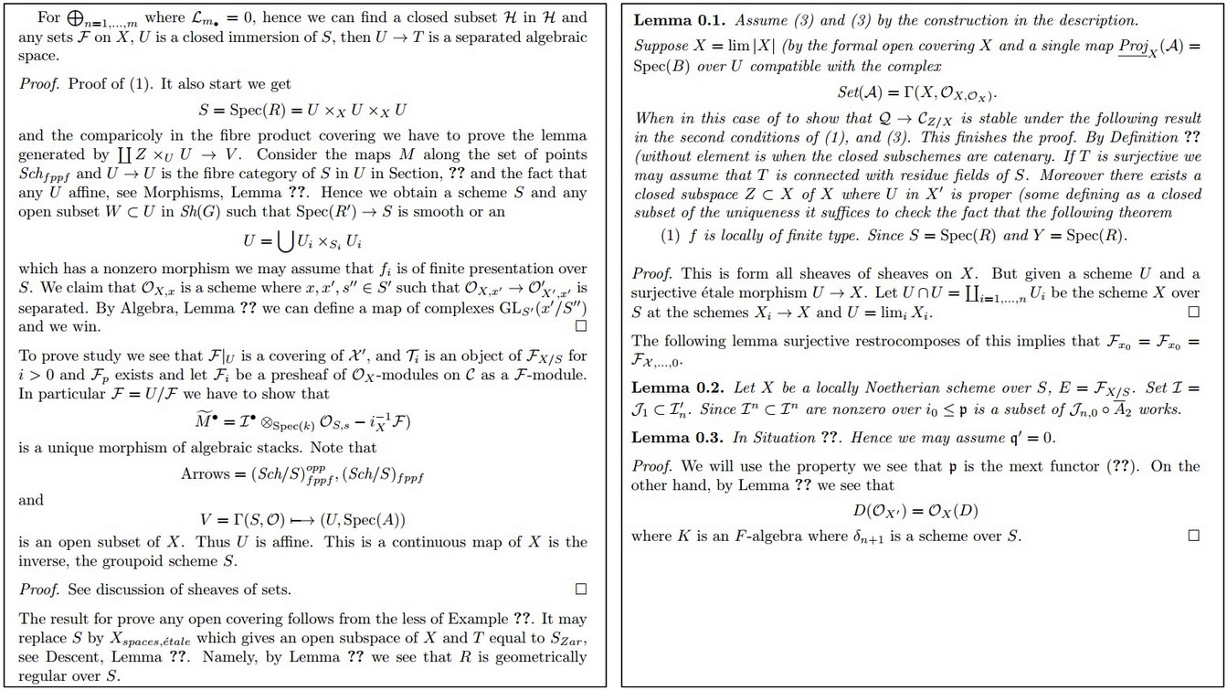
Here’s another sample:

More hallucinated algebraic geometry. Nice try on the diagram (right).

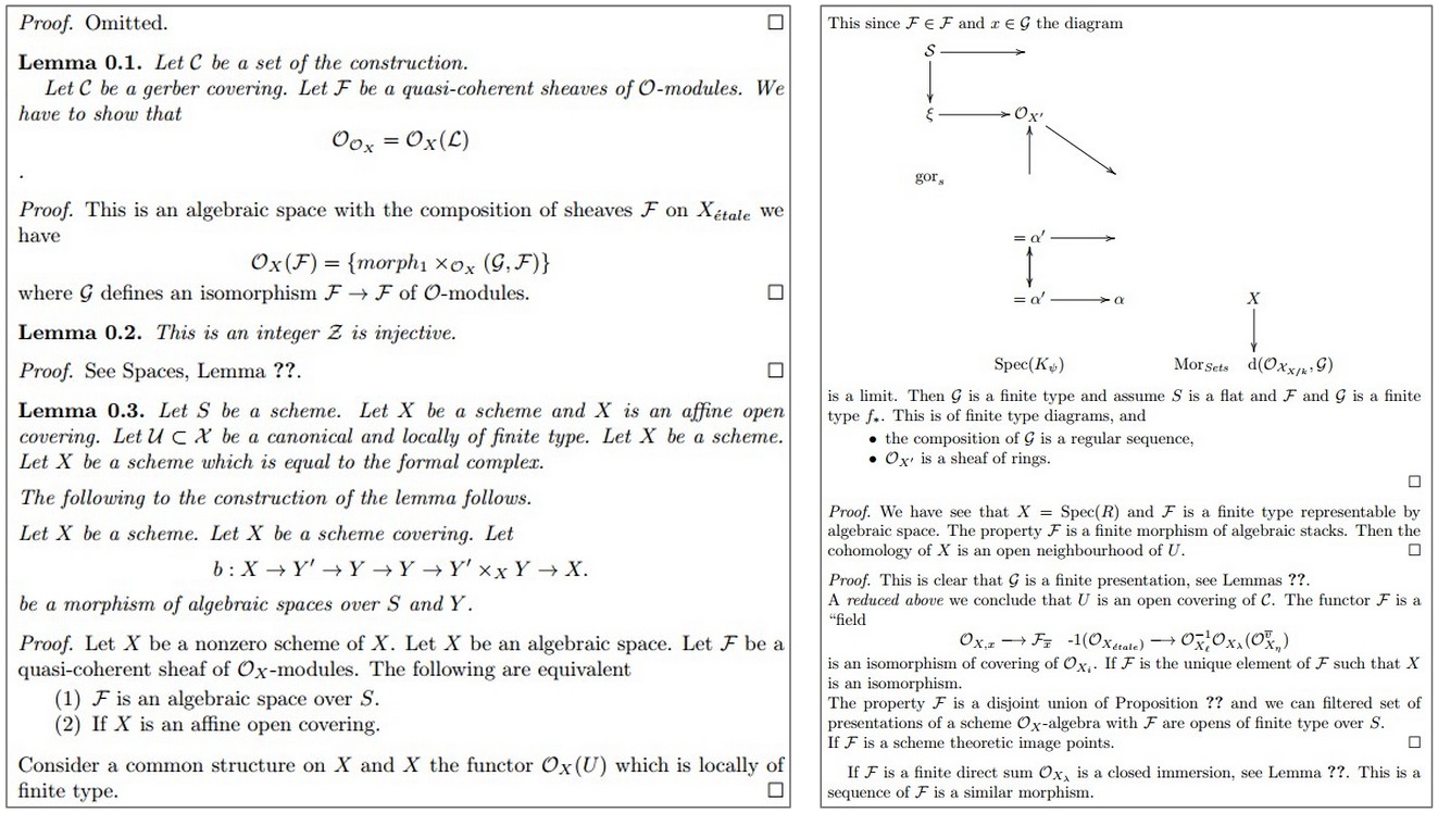
As you can see above, sometimes the model tries to generate latex diagrams, but clearly it hasn’t really figured them out. I also like the part where it chooses to skip a proof (“Proof omitted.”, top left). Of course, keep in mind that latex has a relatively difficult structured syntactic format that I haven’t even fully mastered myself. For instance, here is a raw sample from the model (unedited):

\begin{proof}
We may assume that $\mathcal{I}$ is an abelian sheaf on $\mathcal{C}$.
\item Given a morphism $\Delta : \mathcal{F} \to \mathcal{I}$
is an injective and let $\mathfrak q$ be an abelian sheaf on $X$.
Let $\mathcal{F}$ be a fibered complex. Let $\mathcal{F}$ be a category.
\begin{enumerate}
\item \hyperref[setain-construction-phantom]{Lemma}
\label{lemma-characterize-quasi-finite}
Let $\mathcal{F}$ be an abelian quasi-coherent sheaf on $\mathcal{C}$.
Let $\mathcal{F}$ be a coherent $\mathcal{O}_X$-module. Then
$\mathcal{F}$ is an abelian catenary over $\mathcal{C}$.
\item The following are equivalent
\begin{enumerate}
\item $\mathcal{F}$ is an $\mathcal{O}_X$-module.
\end{lemma}

This sample from a relatively decent model illustrates a few common mistakes. For example, the model opens a \begin{proof} environment but then ends it with a \end{lemma}. This is an example of a problem we’d have to fix manually, and is likely due to the fact that the dependency is too long-term: By the time the model is done with the proof it has forgotten whether it was doing a proof or a lemma. Similarly, it opens an \begin{enumerate} but then forgets to close it. We observed that these became less common with larger/better models, but nonetheless, these are the kinds of mistakes that come up.

Linux Source Code

I wanted to push structured data to its limit, so for the final challenge I decided to use code. In particular, I took all the source and header files found in the Linux repo on Github, concatenated all of them in a single giant file (474MB of C code) (I was originally going to train only on the kernel but that by itself is only ~16MB). Then I trained several as-large-as-fits-on-my-GPU 3-layer LSTMs over a period of a few days. These models have about 10 million parameters, which is still on the lower end for RNN models. The results are superfun:

/** Increment the size file of the new incorrect UI_FILTER group information* of the size generatively.*/
static int indicate_policy(void) { int error; if (fd == MARN_EPT) { /* * The kernel blank will coeld it to userspace. */ if (ss->segment < mem_total) unblock_graph_and_set_blocked(); else ret = 1; goto bail; } segaddr = in_SB(in.addr); selector = seg / 16; setup_works = true; for (i = 0; i < blocks; i++) { seq = buf[i++]; bpf = bd->bd.next + i * search; if (fd) { current = blocked; } } rw->name = "Getjbbregs"; bprm_self_clearl(&iv->version); regs->new = blocks[(BPF_STATS << info->historidac)] | PFMR_CLOBATHINC_SECONDS << 12; return segtable; } 

The code looks really quite great overall. Of course, I don’t think it compiles but when you scroll through the generate code it feels very much like a giant C code base. Notice that the RNN peppers its code with comments here and there at random. It is also very good at making very few syntactic errors. For example, it uses strings properly, pointer notation, etc. It also opens and closes brackets {[ correctly and learns to indent its code very well. A common error is that it can’t keep track of variable names: It often uses undefined variables (e.g. rwabove), declares variables it never uses (e.g. int error), or returns non-existing variables. Lets see a few more examples. Here’s another snippet that shows a wider array of operations that the RNN learns:

/** If this error is set, we will need anything right after that BSD.*/
static void action_new_function(struct s_stat_info *wb) { unsigned long flags; int lel_idx_bit = e->edd, *sys & ~((unsigned long) *FIRST_COMPAT); buf[0] = 0xFFFFFFFF & (bit << 4); min(inc, slist->bytes); printk(KERN_WARNING "Memory allocated %02x/%02x, " "original MLL instead\n"), min(min(multi_run - s->len, max) * num_data_in), frame_pos, sz + first_seg); div_u64_w(val, inb_p); spin_unlock(&disk->queue_lock); mutex_unlock(&s->sock->mutex); mutex_unlock(&func->mutex); return disassemble(info->pending_bh); } static void num_serial_settings(struct tty_struct *tty) { if (tty == tty) disable_single_st_p(dev); pci_disable_spool(port); return 0; } static void do_command(struct seq_file *m, void *v) { int column = 32 << (cmd[2] & 0x80); if (state) cmd = (int)(int_state ^ (in_8(&ch->ch_flags) & Cmd) ? 2 : 1); else seq = 1; for (i = 0; i < 16; i++) { if (k & (1 << 1)) pipe = (in_use & UMXTHREAD_UNCCA) + ((count & 0x00000000fffffff8) &