Gradient boosting is a powerful machine learning algorithm used to achieve state-of-the-art accuracy on a variety of tasks such as regression, classification and ranking. It has achieved notice in machine learning competitions in recent years by “winning practically every competition in the structured data category”. If you don’t use deep neural networks for your problem, there is a good chance you use gradient boosting.

In this post I look at the popular gradient boosting algorithm XGBoost and show how to apply CUDA and parallel algorithms to greatly decrease training times in decision tree algorithms. I originally described this approach in my MSc thesis and it has since evolved to become a core part of the open source XGBoost library as well as a part of the H2O GPU Edition by H2O.ai.

H2O GPU Edition is a collection of GPU-accelerated machine learning algorithms including gradient boosting, generalized linear modeling and unsupervised methods like clustering and dimensionality reduction. H2O.ai is also a founding member of the GPU Open Analytics Initiative, which aims to create common data frameworks that enable developers and statistical researchers to accelerate data science on GPUs.

Gradient Boosting

The term “gradient boosting” comes from the idea of “boosting” or improving a single weak model by combining it with a number of other weak models in order to generate a collectively strong model. Gradient boosting is an extension of boosting where the process of additively generating weak models is formalised as a gradient descent algorithm over an objective function.

Gradient boosting is a supervised learning algorithm. This means that it takes a set of labelled training instances as input and builds a model that aims to correctly predict the label of each training example based on other non-label information that we know about the example (known as features of the instance). The purpose of this is to build an accurate model that can automatically label future data with unknown labels.

Table 1 shows a toy dataset with four columns: ”age”, “has job”, “owns house” and “income”. In this example I will use income as the label (sometimes known as the target variable for prediction) and use the other features to try to predict income.

To do this, first I need to come up with a model, for which I will use a simple decision tree. Many different types of models can be used for gradient boosting, but in practice decision trees are almost always used. I’ll skip over exactly how the tree is constructed. For now it is enough to know that it can be constructed in order to greedily minimise some loss function (for example squared error).

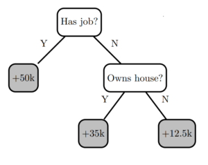Figure 1. Decision tree 0.

Figure 1 shows a simple decision tree model (I’ll call it “Decision Tree 0”) with two decision nodes and three leaves. A single training instance is inserted at the root node of the tree, following decision rules until a prediction is obtained at a leaf node.

This first decision tree works well for some instances but not so well for other instances. Subtracting the predicted label () from the true label () shows whether the prediction is an underestimate or an overestimate. This is called the residual and is denoted as :

.

Table 2 shows the residuals for the dataset after passing its training instances through tree 0.

Figure 2. Decision tree 1.

To improve the model, I can build another decision tree, but this time try to predict the residuals instead of the original labels. This can be thought of as building another model to correct for the error in the current model.

I add the new tree to the model, make new predictions and then calculate residuals again. In order to make predictions with multiple trees I simply pass the given instance through every tree and sum up the predictions from each tree.

Let’s take a look at the sum of squared errors for the extended model. SSE can be calculated as:

.

For the baseline model I just predict 0 for all instances.

You can see that the error decreases as new models are added. To explain why fitting new models to the residuals of the current model increases the performance of the complete model, take the gradient of the SSE loss function for a single training instance:

.

So the residual  is the negative gradient of the loss function for this training instance. Hence, by building models that adjust labels in the direction of these residuals, this is actually a gradient descent algorithm on the squared error loss function for the given training instances.

This minimises the loss function for the training instances until it eventually reaches a local minimum for the training data.

The XGBoost Algorithm

The above algorithm describes a basic gradient boosting solution, but a few modifications make it more flexible and robust for a variety of real world problems.

In particular, XGBoost uses second-order gradients of the loss function in addition to the first-order gradients, based on Taylor expansion of the loss function. You can take the Taylor expansion of a variety of different loss functions (such as logistic loss for binary classification) and plug them into the same algorithm for greater generalisation.

In addition to this, XGBoost transforms the loss function into a more sophisticated objective function containing regularisation terms. This extension of the loss function adds penalty terms for adding new decision tree leaves to the model with penalty proportional to the size of the leaf weights. This inhibits the growth of the model in order to prevent overfitting. Without these regularisation terms, gradient boosted models can quickly become large and overfit to noise present in the training data. Overfitting means that the model may look very good on the training set but generalises poorly to new data that it has not seen before.

You can find a more detailed mathematical explanation of the XGBoost algorithm in the documentation.

Quantiles

In order to explain how to formulate a GPU algorithm for gradient boosting, I will first compute quantiles for the input features (‘age’, ‘has job’, ‘owns house’). This process involves finding cut points that divide a feature into equal-sized groups. The boolean features ‘has job’ and ‘owns house’ are easily transformed by using 0 to represent false and 1 to represent true. The numerical feature ‘age’ transforms into four different groups.

The following table shows the training data with quantised features.

It turns out that dealing with features as quantiles in a gradient boosting algorithm results in accuracy comparable to directly using the floating point values, while significantly simplifying the tree construction algorithm and allowing a more efficient implementation.

Finding Splits in Decision Trees

Here’s a brief explanation of how to find appropriate splits for a decision tree, assuming SSE is the loss function. As an example, I’ll try to find a decision split for the “age” feature at the start of the boosting process. After quantisation there are three different possible splits I could create for this feature: (age < 18), (age < 32) or (age < 67). I need a way to evaluate the quality of each of these splits with respect to the loss function in order to pick the best.

Given a node in a tree that currently contains a set of training instances  and makes a prediction  (this prediction value is also called the leaf weight), I can re-express the loss function at boosting iteration  as follows with  as the prediction so far for instance  and  as the weight predicted for that instance in the current tree:

.

Rewritten in terms of the residuals and expanded this yields

.

I can simplify here by denoting the sum of residuals in the leaf  as .

.

The above equation gives the training loss of a set of instances in a leaf. The next question is, what value should I predict in this leaf to minimise the loss function? The optimal leaf weight  is given by setting

.

This gives

.

I can plug this back into the loss function for the current boosting iteration to see the effect of predicting  in this leaf:

.

Simplifying, I get

.

This equation tells what the training loss will be for a given leaf , but how does it tell me if one split is better than another? When I create a split in the training instances , I denote the set of instances going down the left branch as  and those going down the right branch . I predict  in the left leaf and  in the right leaf.

.

The above equation gives the training loss for a given split in the tree, so I can simply apply this function to a number of possible splits under consideration and choose the one with the lowest training loss. I can recursively create new splits down the tree until I reach a specified depth or other stopping condition.

Note that the sum term  never actually changes at boosting iteration  and can be ignored for the purpose of determining if one split is better than another in the current tree. This means that, despite all of the equations, I only need the sum of the residuals in the left-hand branch (), the sum of the residuals in the right-hand branch () and the number of examples in each (, ) to evaluate the relative quality of a split. I call this reduced function the “split loss”:

.

Implementation: Histograms and Prefix Sums

Bringing this back to my example of finding a split for the feature “age”, I’ll start by summing the residuals for each possible quantile value of age. Assume I’m at the start of the boosting process and therefore the residuals  are equivalent to the original labels .

The sums for each quantile can be calculated easily in CUDA using simple global memory atomic add operations or using the more sophisticated shared memory histogram algorithm discussed in this post.

In order to apply the  function, I need to know the sum of all values to the left and all values to the right of possible split points. To do this I can use the ever useful parallel prefix sum (or scan) operation. In this case I use the “inclusive” variant of scan for which efficient implementations are available in the thrust and cub libraries. I also make the reasonable assumption that I know the sum of all residuals in the current set of instances (210 here). This allows me to calculate the sum of elements to the right by subtracting the elements to the left (the inclusive scan) from the total.

Quantile	<18	<32	<67	67+
	1	2	2	1
Quantile sum	0	60	115	35
Inclusive scan	1	3	5	6
Inclusive scan	0	60	175	210
Split loss	-4410	-4350	-3675	–

After applying the split loss function to the dataset, the split (<18) has the greatest reduction in the SSE loss function.

I would also perform this test over all other features and then choose the best out of all features to create a decision node in the tree. A GPU can do this in parallel for all nodes and all features at a given level of the tree, providing powerful scalability compared to CPU-based implementations.

Memory Efficiency: Bit Compression and Sparsity

Gradient boosting in XGBoost contains some unique features specific to its CUDA implementation. Memory efficiency is an important consideration in data science. Datasets may contain hundreds of millions of rows, thousands of features and a high level of sparsity. Given that device (GPU) memory capacity is typically smaller than host (CPU) memory, memory efficiency is important.

I have implemented parallel primitives for processing sparse CSR (Compressed Sparse Row) format input matrices following work in the modern GPU library and CUDA implementation of sparse matrix vector multiplication algorithms. These primitives allow me to process a sparse matrix in CSR format with one work unit (thread) per non-zero matrix element and efficiently look up the associated row index of the non-zero element using a form of vectorised binary search. This significantly reduces storage requirements, provides stable performance and still allows very clean and readable code.

Another innovation is the use of symbol compression to store the quantised input matrix on the device. The maximum integer value contained in a quantised nonzero matrix element is proportional to the number of quantiles, commonly 256, and to the number of features which are specified at runtime by the user. It seems wasteful to use a four-byte integer to store a value that very commonly has a maximum value less than 216. To solve this, the input matrix is bit compressed down to  bits per element on the host before copying it to the device. Note that this data is not modified once on the device and is read many times.

I can then define an iterator that accesses these compressed elements in a seamless way, resulting in minimal changes to existing CUDA kernels and function calls:

CompressedIterator<int> itr(compressed_buffer, max_value); template <typename iter_t> __global__ void some_kernel(iter_t x) { int tid = threadIdx.x + blockIdx.x * blockDim.x; int decompressed_value = x[tid]; }

It’s easy to implement this compressed iterator to be compatible with the Thrust library, allowing the use of parallel primitives such as scan:

thrust::device_vector<int> output(n); thrust::exclusive_scan(itr, itr + n, output.begin());

Using this bit compression method in XGBoost reduces the memory cost of each matrix element to less than 16 bits in typical use cases. This is half the cost of the equivalent CPU implementation. Note that while it would be possible to use this iterator just as easily on the CPU, the instructions required to extract a symbol from the compressed stream can result in a noticeable performance penalty. The GPU kernels are typically memory bound (as opposed to compute bound) and therefore do not incur the same performance penalty from extracting symbols.

Performance on GPUs

I evaluate performance of the entire boosting algorithm using the commonly benchmarked UCI Higgs dataset. This is a binary classification problem with 11M rows * 29 features and is a relatively time consuming problem in the single machine setting.

The following Python script runs the XGBoost algorithm. It outputs the decreasing test error during boosting and measures the time taken by GPU and CPU algorithms.

import csv
import numpy as np import os.path import pandas import time import xgboost as xgb import sys if sys.version_info[0] >= 3: from urllib.request import urlretrieve else: from urllib import urlretrieve data_url = "https://archive.ics.uci.edu/ml/machine-learning-databases/00280/HIGGS.csv.gz" dmatrix_train_filename = "higgs_train.dmatrix" dmatrix_test_filename = "higgs_test.dmatrix" csv_filename = "HIGGS.csv.gz" train_rows = 10500000 test_rows = 500000 num_round = 1000 plot = True # return xgboost dmatrix def load_higgs(): if os.path.isfile(dmatrix_train_filename) and os.path.isfile(dmatrix_test_filename): dtrain = xgb.DMatrix(dmatrix_train_filename) dtest = xgb.DMatrix(dmatrix_test_filename) if dtrain.num_row() == train_rows and dtest.num_row() == test_rows: print("Loading cached dmatrix...") return dtrain, dtest if not os.path.isfile(csv_filename): print("Downloading higgs file...") urlretrieve(data_url, csv_filename) df_higgs_train = pandas.read_csv(csv_filename, dtype=np.float32, nrows=train_rows, header=None) dtrain = xgb.DMatrix(df_higgs_train.ix[:, 1:29], df_higgs_train[0]) dtrain.save_binary(dmatrix_train_filename) df_higgs_test = pandas.read_csv(csv_filename, dtype=np.float32, skiprows=train_rows, nrows=test_rows, header=None) dtest = xgb.DMatrix