With the theory done, we can now teleport a real qubit on a real device!

理论完成后，我们现在可以在真实设备上传送真实的量子比特！

This is the second part of my series on quantum teleportation. The first part covers the basics of quantum computing and ends with a description of the circuit which we will be using in this article. In this part, we will pick up there and learn how to code it using a python package qiskit. Along the way, you’ll also learn a bit about some of the current challenges in quantum computing. If you feel confused at any point, have another read of the first part or ask me in the questions!

这是我关于量子隐形传态系列的第二部分。 第一部分涵盖了量子计算的基础知识，并以对本文将要使用的电路的描述作为结尾。 在这一部分中，我们将在那里学习并学习如何使用python软件包qiskit对其进行编码。 在此过程中，您还将学到一些有关量子计算当前挑战的知识。 如果您在任何时候感到困惑，请再次阅读第一部分或在问题中问我！

Prerequisites:

先决条件：

• Python and Jupyter notebook installed安装了Python和Jupyter笔记本

• An IBMQ account

  一个IBMQ帐户

• Familiarity with quantum computing notation and the circuit below熟悉量子计算符号和下面的电路
• A pair of red socks with at least one hole in一双至少有一个洞的红色袜子

So this is the magic circuit:

这就是魔术电路：

To summarise:

总结一下：

• Alice and Bob share a Bell pair, β₀₀.爱丽丝和鲍勃共享一个贝尔对，β₀₀。
• Alice wants to send an arbitrary qubit, ψ, to Bob.爱丽丝想向鲍勃发送一个任意的量子比特ψ。
• Alice has the top two qubits in the diagram, Bob has the bottom one.爱丽丝在图中的前两个量子位，鲍勃在下一个。
• Alice applies two gates to her qubits.爱丽丝对她的量子位应用了两个门。
• Alice measures her qubits and sends the results (classically) to Bob.爱丽丝测量她的量子位，并将结果(经典地)发送给鲍勃。
• Bob applies the appropriate corrections and recovers ψ!鲍勃应用适当的更正并恢复ψ！

奇斯奇 (Qiskit)

This tutorial will be programmed in qiskit. Qiskit is an open-source python package developed by IBM. It makes the creation and simulation of quantum circuits extremely easy. You can also send your circuits to one of IBM’s 9 publically available quantum computers, as you’ll see later.

本教程将在qiskit中进行编程。 Qiskit是IBM开发的开源python软件包。 它使量子电路的创建和仿真变得非常容易。 您还可以将电路发送到IBM的9台公开可用的量子计算机之一，这将在以后看到。

To install qiskit, open terminal/cmd and type:

要安装qiskit，请打开terminal / cmd并输入：

pip install qiskit

pip install qiskit

Then open a new jupyter notebook (you can do this in any python environment, but jupyter is the best way to follow along).

然后打开一个新的jupyter笔记本(您可以在任何python环境中执行此操作，但是jupyter是最好的方法)。

Our first disappointment of the article is that we are not actually going to teleport a qubit very far. The current technology only allows us to run a single circuit on a single quantum computer at any one time and so we will only be teleporting our qubit from the top of the circuit to the bottom. You will have to pretend that Alice and Bob separate themselves after creating their Bell pair.

我们对本文的第一个失望是，我们实际上并不会远距离传送量子比特。 当前的技术仅允许我们在任何时间在一台量子计算机上运行单个电路，因此我们只能将量子位从电路的顶部传送到电路的底部。 您将不得不假装爱丽丝(Alice)和鲍勃(Bob)在创建贝尔对之后将自己分开。

So to create our lonesome circuit, import qiskit and create a 3 qubit circuit as follows:

因此，要创建我们的寂寞电路，请导入qiskit并创建一个3 qubit电路，如下所示：

from qiskit import QuantumCircuit

from qiskit import QuantumCircuit

qc = QuantumCircuit(3)

qc = QuantumCircuit(3)

Simple as that! To see it type qc.draw() and you should see:

就那么简单！ 要查看它，请键入qc.draw() ，您应该看到：

Unsurprisingly, not a lot going on so far. We can, however, see that the qubits are labelled q_0, q_1 and q_2. We would prefer to distinguish between Alice’s and Bob’s qubits. To do that we need to create separate ‘quantum registers’ which can be named anything. We’ll make one for Alice (with 2 qubits) and one for Bob (with 1 qubit). To do that type:

不足为奇的是，到目前为止没有发生太多事情。 但是，我们可以看到这些量子位被标记为q_0，q_1和q_2。 我们希望区分爱丽丝和鲍勃的量子位。 为此，我们需要创建单独的“量子寄存器”，可以将其命名为任何东西。 我们将为Alice(带有2个量子比特)制作一个，为Bob(带有1个量子比特)制作一个。 为此，请输入：

from qiskit import QuantumRegisteralice_reg = QuantumRegister(2, name="alice")bob_reg = QuantumRegister(1, name="bob")qc = QuantumCircuit(alice_reg, bob_reg)qc.draw()

This should give:

这应该给出：

This looks a bit cumbersome, so change the last line to qc.draw(output='mpl') and it will format the diagram much more nicely:

这看起来有点麻烦，所以将最后一行更改为qc.draw(output='mpl') ，它将使图表的格式更加美观：

We are finally ready to apply some gates.

我们终于准备好要施加一些条件了。

准备铃对 (Preparing Bell Pair)

The first step in our protocol is for Alice and Bob to share a Bell pair. Remember from my first article to that to prepare a Bell pair we use the |+> state as a control in a CNOT and 0 as the target. In qiskit, that’s as simple as telling it which operations to apply on which qubits:

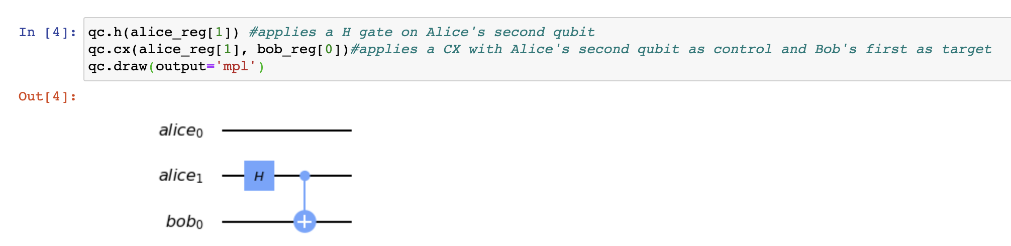
我们协议的第一步是让Alice和Bob共享一个Bell对。 请记住，在我的第一篇文章中，要准备一个贝尔对，我们在CNOT中使用| +>状态作为控件，并使用0作为目标。 在qiskit中，这很简单，只要告诉它在哪些qubit上应用哪些操作即可：

qc.h(alice_reg[1]) qc.cx(alice_reg[1], bob_reg[0])

Drawing the circuit should now give:

现在绘制电路应该给出：

Remember how last time I mentioned that measuring a Bell pair many times will randomly give 00 and 11, but never anything else? Remember that Einstein wasn’t so convinced? Well, let’s test it!

还记得我上次提到多次测量一个贝尔对会随机给出00和11，但没有别的什么吗？ 还记得爱因斯坦不那么相信吗？ 好吧，让我们测试一下！

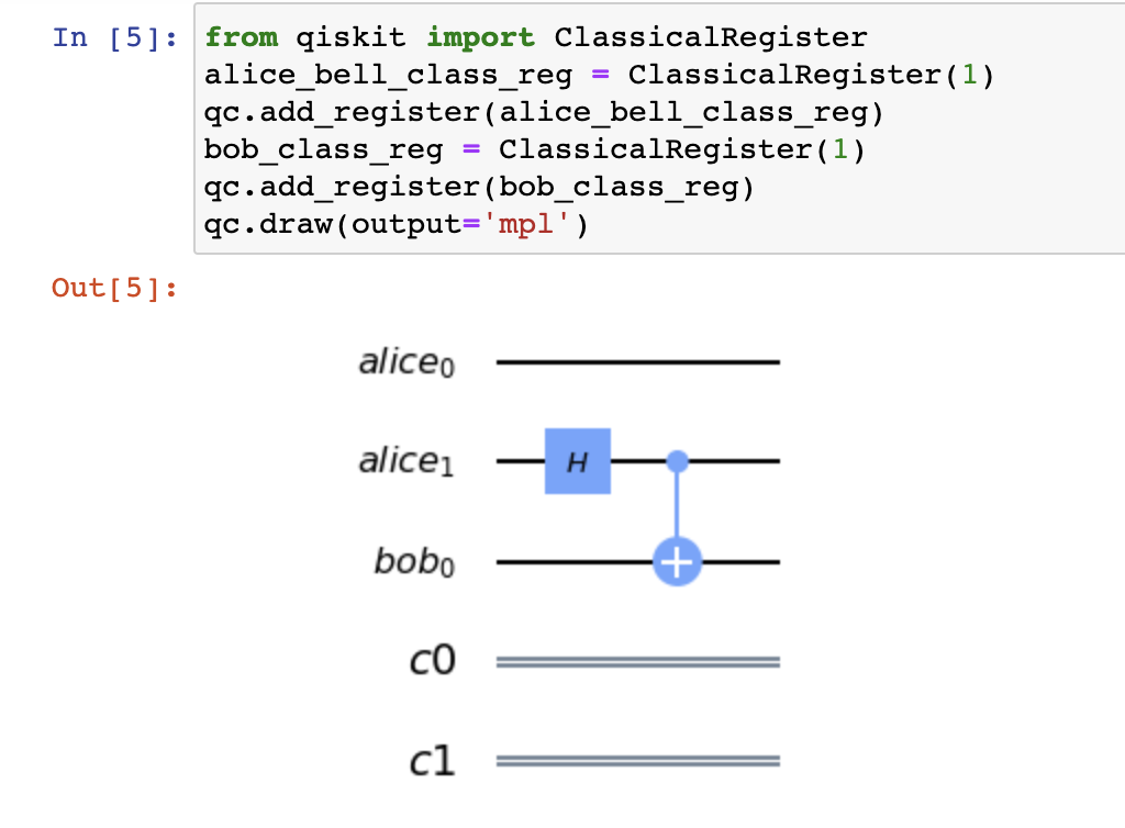
All we need to do measure the qubits. To do that we‘ll create some ClassicalRegisters and add them to the circuit (there are easier ways to do this, but we have to do it this way, for now, to allow the measurement results to be used in the circuit later on).

我们所需要做的就是测量量子位。 为此，我们将创建一些ClassicalRegisters并将其添加到电路中(有更简单的方法，但是现在我们必须以这种方式进行操作，以允许稍后在电路中使用测量结果) 。

from qiskit import ClassicalRegisteralice_bell_class_reg = ClassicalRegister(1)qc.add_register(alice_bell_class_reg)bob_class_reg = ClassicalRegister(1)qc.add_register(bob_class_reg)

This adds the classical registers to the bottom of the circuit:

这将经典寄存器添加到电路的底部：

And then to measure the results, simply do:

然后要测量结果，只需执行以下操作：

qc.measure(alice_reg[1], alice_bell_class_reg) #measures Alice's second qubit into the first classical bitqc.measure(bob_reg[0], bob_class_reg) #measures Bob's first qubit in the second classical bit

Then we can either simulate the circuit or run it on a real device.

然后，我们可以仿真电路或在真实设备上运行它。

To simulate our circuit:

模拟我们的电路：

from qiskit import BasicAer, executebackend = BasicAer.get_backend('qasm_simulator')results = execute(qc, backend=backend).result()results.get_counts()

This simulates the circuit 1024 times by default and gives me:

默认情况下，这会模拟电路1024次，并为我提供：

So we see that we have roughly random proportions of 00 and 11! Suck on that, local realism.

因此，我们看到我们大约有00和11的随机比例！ 吸纳当地的现实主义。

“Nay”, say you naysayers, “you have only simulated it. The qubits are even right next to each other. Show me the real deal”. Have patience my friends, all in good time. Unfortunately, the technology is not yet ready for us to separate these qubits very far either, as their lifetime is around 100μs. And yes, while it is true that this is a mere simulation, see here for a comprehensive list of the times that it has been experimentally verified outside of a quantum computer.

反对者说：“不，”您只是模拟了它。 量子位甚至彼此相邻。 告诉我真正的交易”。 朋友们，请耐心等待，一切顺利。 不幸的是，由于它们的寿命约为100μs，因此我们还没有准备好将这些量子比特分离得很远。 是的，虽然这确实是单纯的模拟，但请参阅此处 ，以获取在量子计算机之外进行实验验证的完整时间列表。

Still not good enough for you? Alright then, let’s run it on the real thing.

还不够适合您吗？ 好吧，让我们在真实的东西上运行它。

The first step is to link your IBMQ account with your qiskit (I’ve obviously not shown you my key, and I’ve stored in the past so yours should say something different):

第一步是将您的IBMQ帐户与qiskit关联(我显然没有给您显示我的密钥，并且我已经存储了过去，所以您的说法应该有所不同)：

You can then see what devices are available for you:

然后，您可以查看可用的设备：

IBMQ.load_account()provider = IBMQ.get_provider(hub='ibm-q')provider.backends()

This corresponds to the list of devices on the IBM quantum experience website:

这对应于IBM Quantum Experience网站上的设备列表：

So all we need to do is choose a device and send it off. I’m going to choose the least busy.

因此，我们要做的就是选择一台设备并将其发送出去。 我要选择最不忙的人。

# get the least-busy backend at IBM and run the quantum circuit therefrom qiskit.providers.ibmq import least_busybackend = least_busy(provider.backends(simulator=False))print(backend)job_exp = execute(qc, backend=backend, shots=1024)exp_result = job_exp.result()exp_measurement_result = exp_result.get_counts(qc)print(exp_measurement_result)

Here is what I got:

这是我得到的：

Uh oh, it’s not just 00 and 11 :( . I can hear those naysayers, with newfound confidence and a hint of smugness, telling me “you kept promising we’d get these magic results but as soon as you do it on a real quantum computer it fails, screw you man”. At first glance, it does indeed seem like I’ve been leading you on like absolute mugs. Luckily for both of us, that’s not the case.

嗯，不只是00和11 :(。我可以听到那些反对者，充满新的信心和自鸣得意地告诉我：“您一直保证我们会得到这些神奇的结果，但只要您真正做到这一点，乍一看，确实看起来像是我像绝对的水杯一样带领着你。幸运的是，对于我们俩来说，事实并非如此。

Plotting the histogram of the results shows that we did what we were hoping did happen most of the time:

绘制结果的直方图表明，我们做了我们希望在大多数情况下都会发生的事情：

The rare occurrences of 01 and 10 are, unfortunately, due to errors in the quantum computer. Error rates on quantum computers are still very real problems. When I ran my circuit, it was executed on ‘ibmq_vigo’. Clicking on that device on the IBM quantum experience website, it shows me this information:

不幸的是，01和10的罕见出现是由于量子计算机中的错误。 量子计算机上的错误率仍然是非常实际的问题。 当我运行电路时，它是在“ ibmq_vigo”上执行的。 在IBM Quantum Experience网站上单击该设备，它将向我显示以下信息：

This diagram tells me how many qubits the device has, which qubits can be connected by CNOTS (the arrows) and the typical error rates (the colours). The CNOT error rates are therefore between 7/10³ and 2/10² so its not that surprising that we had 70 (52 + 18) errors out of 1024 runs of the circuit. Of course, there is a lot of work going into decreasing these errors and it will be very interesting to see how much better they will be in just a years time (why not share this article with all your friends so they remind you to read it again then?)

该图告诉我设备有多少个量子位，可以通过CNOTS(箭头)和典型的错误率(颜色)来连接哪些量子位。 因此，CNOT的错误率在7 /10³和2 /10²之间，因此，在电路的1024条运行中，我们有70(52 + 18)个错误，这并不奇怪。 当然，要减少这些错误，还有很多工作要做，并且很高兴看到它们在短短的一年内会变得更好(为什么不与所有朋友分享这篇文章，所以他们提醒您阅读它)然后呢？)

Alright so there you are, you have performed real magic on a real quantum computer, admittedly with some errors along the way.

好的，您就已经在真实的量子计算机上执行了真正的魔术，顺便提了一些错误。

准备ψ (Preparing ψ)

The second step in our protocol is for Alice to have the qubit ψ. The whole point of ψ is that it could be anything. In our example, we’ll make it applying a quarter of an X gate. An X gate is implemented as a rotation on the x-axis, known as rx, by angle π and so to do a quarter of that we can just do and rx rotation by π/4 (feel free to apply any amount you would like). We will apply it on Alice’s first qubit. We’ll also add a classical register to measure it into later

我们协议的第二步是让Alice具有qubitψ。 ψ的全部要点是可以是任何东西。 在我们的示例中，我们将使其应用X门的四分之一。 X闸门实现为在x轴上的旋转，称为rx，旋转角度为π，因此要做到四分之一，我们可以做，而rx旋转π/ 4(可以随意应用您想要的任何量)。 我们将其应用于爱丽丝的第一个量子位。 我们还将添加一个经典的寄存器以供以后使用

from math import piqc.rx(pi/4, alice_reg[0])alice_psi_class_reg = ClassicalRegister(1)qc.add_register(alice_psi_class_reg)

Now restart your kernel and run your code again from the beginning, missing out the cells which measured, simulated and ran the circuit as we don’t want to destroy our precious Bell pair quite yet. Adding a barrier to separate our stages then drawing the circuit again, you should now see:

现在，重新启动内核，并从头开始重新运行代码，因为我们还不想破坏我们宝贵的贝尔对，所以错过了进行测量，模拟和运行电路的单元。 添加一个障碍物以分隔各个阶段，然后再次绘制电路，您现在应该看到：

To see what the effect of that Rx gate is, I’m going to measure the first qubit and simulate it a few times. I’ll show my results so you don’t need to code this bit if you don’t want.

为了了解Rx门的作用，我将测量第一个qubit并对其进行几次仿真。 我将显示结果，以便您不需要时也无需编写代码。

We get mostly zeros with a few ones (don’t worry about the exact ratio or the second two qubits since we haven’t measured them). But if we apply an Rx gate with an angle -π/4, we’ll return to more consistent results.

我们得到的零多数为零(不要担心确切的比率或后两个qubit，因为我们没有测量它们)。 但是，如果我们应用角度为-π/ 4的Rx门，我们将返回更一致的结果。

Alright lovely stuff, so the plan is to apply this -π/4 rotation on the third qubit after we’ve done the teleportation, fixing it back to zero.

好的东西，所以计划是在完成隐形传送后在第三个量子比特上应用此-π/ 4旋转，并将其固定为零。

实际电路 (The actual circuit)

In terms of our circuit diagram, we are now at ψ₀. So all we need to do is apply our two gates:

就电路图而言，现在为ψ₀。 因此，我们需要做的就是应用两个门：

qc.cx(alice_reg[0], alice_reg[1])qc.h(alice_reg[0])

Adding some more barriers for aesthetic convenience and drawing we now have:

为美观方便和绘图添加更多障碍，我们现在拥有：

Next, we’ll measure Alice’s qubits and then to send the information, you can use qiskit.c_ifas follows:

接下来，我们将测量Alice的量子位，然后发送信息，可以使用qiskit.c_if ，如下所示：

qc.measure(alice_reg[0], alice_psi_class_reg)qc.measure(alice_reg[1], alice_bell_class_reg)qc.x(bob_reg[0]).c_if(alice_bell_class_reg, 1) # Apply X to Bob if 2nd qubit measured to 1qc.z(bob_reg[0]).c_if(alice_psi_class_reg, 1) # Apply Z if 1st qubit measured to 1

This adds these special lines to the circuit, which correspond to the double lines in our original circuit diagram:

这会将这些特殊线添加到电路中，这对应于我们原始电路图中的双线：

The qubit has now been teleported and recovered! Finally, we’ll apply that -π/4 gate to ensure we measure zeros and then measure Bob’s qubit:

量子位现在已经被传送和恢复了！ 最后，我们将应用-π/ 4门以确保我们测量零，然后测量Bob的量子比特：

qc.rx(-pi/4, bob_reg[0]qc.measure(bob_reg[0], bob_class_reg)

and simulate:

并模拟：

from qiskit import BasicAer, executebackend = BasicAer.get_backend('qasm_simulator')results = execute(qc, backend=backend).result()results.get_counts()

Here is what I got:

这是我得到的：

The results look pretty random but when comparing to the final circuit diagram:

结果看起来很随机，但与最终电路图相比：

We see that the first and last qubits are the ones used for the correction. These happen randomly. More importantly, notice that the middle qubit is always 0. That is the one we teleported! So not only did we successfully teleport the qubit ψ, but we also correctly recovered it for every combination of Alice’s measurement. Very very cool.

我们看到第一个和最后一个量子位是用于校正的量子位。 这些随机发生。 更重要的是，请注意中间的量子位始终为0。这就是我们所传送的量子位！ 因此，我们不仅成功传送了量子比特ψ，而且还针对Alice测量的每个组合正确地恢复了它。 非常非常酷。

在真实设备上传送 (Teleporting on a real device)

So we are finally ready for the grand finale. Here’s the code again to find a device and run it:

因此，我们终于可以开始大结局了。 这是再次找到设备并运行它的代码：

provider = IBMQ.get_provider(hub='ibm-q')# get the least-busy backend at IBM and run the quantum circuit therefrom qiskit.providers.ibmq import least_busybackend = least_busy(provider.backends(simulator=False))print(backend)job_exp = execute(qc, backend=backend, shots=1024)exp_result = job_exp.result()exp_measurement_result = exp_result.get_counts(qc)print(exp_measurement_result)

And…. it doesn't like it:

和…。 它不喜欢它：

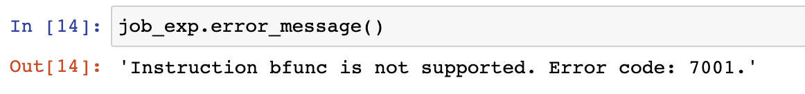
Not a particularly useful error message, but luckily I’m here to tell you that the problem is that we can’t actually use the classical communication channels on real quantum computers yet.

这不是特别有用的错误消息，但是幸运的是，我在这里告诉您的问题是，我们还不能真正在真实的量子计算机上使用经典的通信通道。

So is that it? Time to go home?

就是这样吗？ 该回家了？

Fear not! We can still run the circuit but we will have to make a small compromise. We’re going to have to get rid of the c_if commands and replace them with CNOT and CZ (like a CNOT but performs a Z on the target if control is 1) gates before the measurement of Alice’s gates. Due to something called the principle of deferred measurement, there is actually no observable difference in doing this. However, this does slightly ruin our idea of long-distance teleportation since the qubits have to be connected on a quantum computer to perform these operations. Nevertheless, with current technology that is our only option.

不要怕！ 我们仍然可以运行电路，但是我们必须做出一些小的妥协。 在测量爱丽丝门之前，我们将必须摆脱c_if命令，并用CNOT和CZ代替它们(类似于CNOT，但如果控制为1，则在目标上执行Z)。 由于有一种称为延迟测量的原理 ，因此实际上并没有明显的区别。 但是，由于量子位必须连接到量子计算机上才能执行这些操作，因此这确实会破坏我们的长距离远距传输概念。 不过，采用当前技术是我们唯一的选择。

Since we now no longer need to measure Alice’s qubits, we may as well delete those classical registers. Then, in the block which previously had the c_if operations write:

由于我们现在不再需要测量Alice的量子位，因此我们也可以删除那些经典寄存器。 然后，在先前具有c_if操作的块中编写：

qc.cx(alice_reg[1], bob_reg[0])qc.cz(alice_reg[0], bob_reg[0])

Then restarting the kernel and running again, the entire circuit should now look like:

然后重新启动内核并再次运行，整个电路现在应如下所示：

The gate which looks like two controls is the CZ gate. If you’re wondering how you could tell which is the control, it actually doesn't matter because it adds a sign to the entire state if and only if both qubits are in the 1 state (remember Z|0> does nothing)

看起来像两个控件的门是CZ门。 如果您想知道如何辨别哪个控件，那么实际上并不重要，因为当且仅当两个量子位都处于1状态时，它才向整个状态添加一个符号(记住Z | 0>不执行任何操作)

This circuit we can run on an actual quantum computer. So let’s do it:

我们可以在实际的量子计算机上运行此电路。 因此，让我们做吧：

from qiskit import IBMQIBMQ.load_account()provider = IBMQ.get_provider(hub='ibm-q')from qiskit import executefrom qiskit.providers.ibmq import least_busybackend = least_busy(provider.backends(simulator=False))print(backend)job_exp = execute(qc, backend=backend, shots=1024)exp_result = job_exp.result()exp_measurement_result = exp_result.get_counts(qc)print(exp_measurement_result)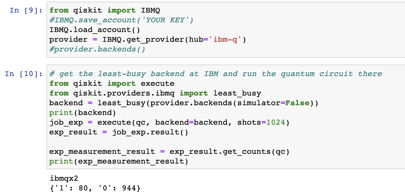

Plotting the histogram of the results:

绘制结果的直方图：

We can see that we got 0 an overwhelming number of times, the small fraction of 1 results being due to errors.

我们可以看到，我们获得0的次数非常多，其中1个结果的一小部分是由于错误造成的。

Congratulations! You have learnt how to teleport a qubit using qiskit on a real quantum computer, with some minor caveats.

恭喜你！ 您已经了解了如何在实际的量子计算机上使用qiskit传送量子比特，但有一些小小的警告。

If you got lost at any point along the way, here is a link to the final circuit code.

如果您在此过程中的任何时候迷路了， 这里是最终电路代码的链接 。

Thanks for reading!

谢谢阅读！

Stay tuned for part 3 of this series, a discussion about how any of this actually works.

请继续关注本系列的第3部分，该部分将讨论其中的实际工作原理。