Check out my WebGL-based wind power simulation demo! Let’s dive into how it works under the hood.

I have an unflattering confession to make: for the last few years working at Mapbox, I avoided direct OpenGL/WebGL programming like a plague. For one reason: the OpenGL API and terminology deeply terrified me. It always looked so complex, confusing, ugly, and verbose that I could never take the plunge and dive into it. I would get an uneasy feeling simply hearing terms like stencil masks, mipmap, depth culling, blend functions, and normal maps.

This year, I decided to finally confront my fears and build something non-trivial with WebGL on my own. 2D wind simulation looked like a perfect opportunity — it’s useful, visually stunning, and challenging, yet it still felt attainable in scope. I was surprised to discover that it was much less scary than it looked!

Wind visualization on the CPU

There are many examples of wind power visualization online, but the most popular and influential one is earth.nullschool.net, a famous project by Cameron Beccario. It’s not open source itself, but it has an old open source version which most other implementations based their code on. One notable open source derivation is Esri Wind-JS. Popular weather services that use the technique include Windy and VentuSky.

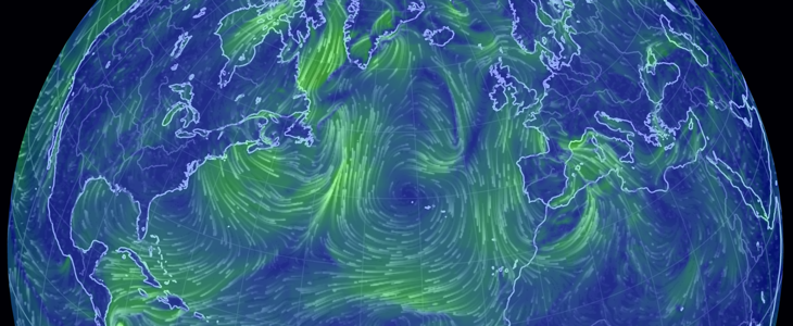
Wind power simulation on earth.nullschool.net

Typically, such a visualization in the browser relies on the Canvas 2D API and roughly works like this:

1. Generate an array of random particle positions on screen and draw the particles.
2. For each particle, query the wind data to get the particle speed in its current location, and move it accordingly.
3. Reset a small portion of particles to a random position. This makes sure that areas the wind blows away from never become fully empty.
4. Fade the current screen a bit and draw newly positioned particles on top.

This has subsequent performance limitations:

• The number of wind particles should be kept low (e.g. Earth uses ~5k).
• There’s a big delay every time you update the data or the view (e.g. ~2 seconds for Earth) because data processing is expensive and happens on the CPU side.

Moreover, to integrate it as a part of an interactive WebGL-based map like Mapbox is that you would have to upload the pixel contents of the Canvas element to the GPU on every frame, which would significantly reduce the performance further.

I was looking for a way to reimplement the full logic on the GPU side with WebGL, so that it would be fast, capable of drawing millions of particles, and possible to integrate into a Mapbox GL map without a big performance loss. Luckily, I stumbled upon a wonderful tutorial about particle physics in WebGLby Chris Wellons, and realized that the wind visualization can use the same approach.

OpenGL Basics

The confusing API and terminology makes OpenGL graphics programming very intimidating to learn, but under the surface, the concept is extremely simple. Here’s a practical definition:

OpenGL provides a 2D API for  drawing triangles  efficiently .

So basically all you do with GL is draw triangles. The difficulty, besides the scary API, comes from the various math and algorithms required to do this. It can also draw dots and basic lines (without smoothing or round joins/caps), but those are rarely used.

Illustration from Brief Introduction to Shaders Using GLSL

OpenGL provides a special C-like language — GLSL — to write programs that are directly executed by the GPU. Each program is divided into two parts, called shaders — the vertex shader and the fragment shader.

The vertex shader provides the code for converting coordinates. For example, multiplying triangle coordinates by 2 so that our triangle appears twice as big. It will run once for every coordinate we pass to OpenGL when drawing. A basic example:

attribute vec2 coord;
void main() {gl_Position = vec4(2.0 * coord, 0, 1);
}

The fragment shader provides the code for determining the color of each drawn pixel. You can do a lot of cool math in it, but in the end it comes down to something like “draw the current pixel of the triangle as green”. Example:

void main() {gl_FragColor = vec4(0, 1, 0, 1);
}

One of the cool things you can do in both vertex and fragment shaders is adding an image (called texture) as a parameter, and then looking up pixel colors in any spot of this image. We’ll rely on this heavily in the wind visualization.

The fragment shader code execution is massively parallel and heavily hardware-accelerated, so it’s usually many orders of magnitude faster than an equivalent computation on the CPU.

Getting the wind data

Every 6 hours, the US National Weather Service publishes weather data for the whole globe, known as GFS, in the form of a latitude/longitude grid with associated values (including wind velocities). It’s encoded in a special binary format called GRIB, which can be parsed into human-readable JSON with a special set of tools.

I wrote a few small scripts that download and convert the wind data into a simple PNG image with wind velocities encoded as RGB colors — horizontal velocity as red and vertical as green in each pixel. It looks like this:

GFS wind power data encoded as an image

There are higher resolution versions you can download (2x and 4x), but 360×180 grid is enough for a low-zoom visualization. PNG compression is quite a good fit for this kind of data, and the image above typically weights just about 80 KB.

Moving particles on the GPU

Existing wind visualizations stored particle state in JavaScript arrays. How do we store and manipulate this state on the GPU side? A new GL feature called compute shaders (in OpenGL ES 3.1 and equivalent WebGL 2.0 specifications) allows you to run shader code on arbitrary data (without any rendering). Unfortunately, support for the new specifications across browsers and mobile devices is marginal, and so we’re left with only one practical option: textures.

OpenGL allows you to draw not only to the screen, but also to a texture (through a concept called framebuffer). So we can encode particle positions as RGBA colors of an image, load it to the GPU, calculate new positions based on wind velocities in the fragment shader, encode them back into RGBA colors and draw it into a new image.

To store enough precision for both X and Y, we store each component in two bytes — RG and BA respectively, giving us a range of 65536 distinct values for each.

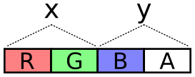
Illustration from A GPU Approach to Particle Physics

An example 500×500 image would then hold 250,000 particles, and we would move every particle with the fragment shader. The resulting image would look like this:

Illustration from A GPU Approach to Particle Physics

Here’s how the position is decoded and encoded from RGBA and back in the fragment shader:

// lookup particle pixel color
vec4 color = texture2D(u_particles, v_tex_pos);

// decode particle position (x, y) from pixel RGBA color
vec2 pos = vec2(color.r / 255.0 + color.b,color.g / 255.0 + color.a);

... // move the position

// encode the position back into RGBA
gl_FragColor = vec4(fract(pos * 255.0),floor(pos * 255.0) / 255.0);

On the next frame, we can take this new image as the current state and draw the new state into the other image, etc., swapping the two every frame. So, with the help of two particle state textures, we can move all the wind simulation logic to the GPU.

This approach is extremely fast — instead of updating only 5,000 particles 60 times per second on the browser, we can suddenly handle one million.

One thing to keep in mind is that near the poles, the particles should move much faster along the X axis compared to the ones on the equator, because the same number of longitude degrees represents a much smaller distance. This can be taken into account with the following shader code:

float distortion = cos(radians(pos.y * 180.0 - 90.0));
// move the particle by (velocity.x / distortion, velocity.y)

Drawing the particles

As I mentioned earlier, in addition to triangles, we can also draw basic points — rarely used, but perfect for 1-pixel particles like this.

To draw each particle, we’ll simply look up its pixel color on the particle state texture in the vertex shader to determine its position; then determine the particle color in the fragment shader by looking up its current velocity from the wind texture; and finally map it to a nice color gradient (I picked the colors from the trusty ColorBrewer2). At this point, it looks like this:

That’s something, if a little empty. But it’s hard to get a sense of wind direction from particle movement alone. We need to add particle trails.

Drawing particle trails

The first approach to drawing the trails I tried is using preserveDrawingBufferWebGL option, which makes the screen state persist between frames, so that we can draw particles over and over on top of each other every frame as they move. However, this WebGL feature is a big performance hit, and many WebGL articles recommend against using it.

Instead, similar to how we do with particle state textures, we can draw the particles into a texture (which is in turn drawn onto a screen), then use this texture on the next frame as the background (slightly dimmed), and swap the input/target textures every frame. In addition to better performance, an advantage of this approach is that we can port it directly to native code (which has no preserveDrawingBuffer equivalent).

Interpolating wind lookups

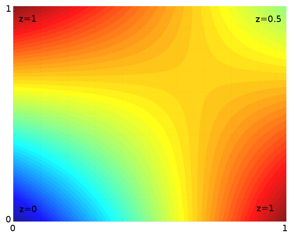
Illustration from a Wikipedia article on Bilinear interpolation

The wind data has values for specific points on a latitude/longitude grid, e.g. (50,30),(51,30),(50,31),(51,31)geographical points. How do we get an arbitrary intermediate value, e.g. (50.123,30.744)?

OpenGL comes with free interpolation when you look up texture colors. However, it’s still leads to blocky, pixelated patterns. Here’s an example of these artifacts in the wind texture when scaled:

Native GL linear interpolation

Luckily, we can smooth out the artifacts by looking up 4 neighbor pixels in each wind probe, and doing manual bilinear interpolation math on them on top of the native one in the fragment shader. It’s more expensive, but fixes the artifacts and leads to a more fluid wind visualization. Here’s the same area with this technique:

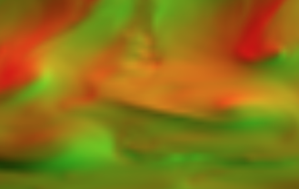
Manual bilinear interpolation on the fragment shader

Pseudo-random generator on the GPU

There’s one tricky logic left to implement on the GPU — randomly resetting particle locations. Without this, even a huge number of wind particles degenerates into just a few lines on the screen, because areas the wind blows away from become empty with time:

The problem is that shaders don’t have a random number generator. How do we randomly decide if a particle needs to be reset?

I found a solution on StackOverflow — a GLSL function for pseudo-random number generation that accepts a pair of numbers as input:

float rand(const vec2 co) {float t = dot(vec2(12.9898, 78.233), co);return fract(sin(t) * (4375.85453 + t));
}

This curious function depends on sin result varying a lot with big values. Then we can do something like this:

if (rand(some_numbers) > 0.99) reset_particle_position();

The challenge is picking an input for each particle that would be “random” enough so that the generated values are uniform across the screen and do not exhibit weird patterns.

Using current particle position as the seed is not perfect because the same particle positions will always generate the same random numbers, so some particles will disappear in the same area.

Using particle position in the state texture also doesn’t work because the same particles will always disappear.

What I ended up with eventually depends on both particle position and state position coupled with a random value that’s calculated on every frame and passed to the shader:

vec2 seed = (pos + v_tex_pos) * u_rand_seed;

But then we have another minor problem — areas where particles are very fast will look much more dense than areas where there’s not much wind. We can balance this out a bit by increasing the particle reset rate for faster particles:

float dropRate = u_drop_rate + speed_t * u_drop_rate_bump;

speed_t here is a relative speed value (from 0 to 1), and u_drop_rate and u_drop_rate_bump are parameters you can tweak in the final visualization. Here's an example of how it affects the result:

High drop rate (reminds me of a Van Gogh painting)

What’s next

The result is a fully GPU-powered wind visualization that can render a million particles at 60fps. Try playing with the sliders in the demo, and check out the final code — it’s about 250 lines total, and I tried to make it as readable as possible.

The next step is integrating this into a live map you can explore. I’ve made some progress on this but not enough to share a live demo. Here’s a little sneak peek though (sorry for the poor quality capture):

Thank you for reading and stay tuned for more updates! And check out my previous article on spatial algorithms if you missed it.

Very special, warm-hearted thank you to my Mapbox team mates @kkaeferand @ansis, who patiently answered all my silly questions about graphics programming, gave tons of valuable tips and helped me learn so much. ❤️

P.S. Want to work on cool stuff like this? Check out our job openings.