r.futures.demand模块决定预期的土地变化总量，它基于历史人口和土地发展数据之间的相关关系，创建了一个需求表格，记录在每个分区的每个步骤上转换的细胞数量。demand使用简单回归计算人口(自变量）和开发地区（因变量）之间的关系，我们甚至可以手动创建一个自定义demand文件，然后使用最合适的方法从运行中获取每一列的值。

• 输入数据：

  • 两景以上来自以往不同年份的 土地发展栅格数据 （1表示已发展，0表示未发展），按照时间顺序进行排列
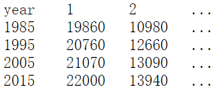
  • 对应于土地发展栅格数据年限的历史分区 人口数据 ，在程序中以observed_population参数表示，输入格式为 *.csv
    • 人口数据的格式表示如下图所示，第一列表示年份（与development参数表示的年份相符合），每一行表示当年内不同分区的人口数据，年份的间隔可以由separator参数来调整。
    • 对于人口预测数据而言，也是同样的文件格式（对应于projected_population参数）

• 注意：
  • 每个分区的代码在三个输入文件中应当是相同的
  • simulation_times参数是一个逗号分隔的年份列表，表示需要被模拟的年份，可以利用python生成这个参数

','.join([str(i) for i in range(2015, 2031)])

• 输出数据：

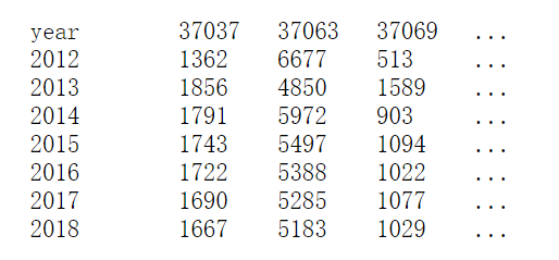
  • 输出的demand表格格式如下图，输出的格式为空格分隔的CSV文件，可以用任意记事本打开
  • 表格中第一列表示年份，其余的列表示一个分区，每一行代表一个年份，表中的每一个值代表该区域每年新发展的细胞数量
  • 注意，当发展需求为负值时（例如人口减少，或需求关系为反比时），demand表中的值设为0，因为模型不会模拟从已发展地区到未发展地区的变化

• 模型模拟

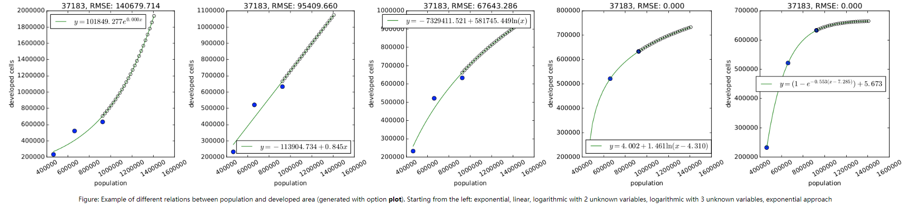
  • 在模型中允许选择人口与已开发地区之间的关系类型，例如线性、对数（2种）、指数、指数逼近等。
  • 如果利用了多种关系类型进行拟合，则使用RMSE选择最佳拟合模型。
  • 推荐的方法有对数法、对数平方法、线性法和指数法，指数法和对数法要求scipy包和至少3个数据点(即三年以上的已发展地区的栅格图)
    • 注：RMSE方法，即（Root Mean Squard Error）均方根误差法，线性回归的损失函数开根号，用来衡量观测值同真值之间的偏差
    • 

• 模拟结果

  • 可以选择输出不同模型模拟结果的散点图，借此可以更有效地评估适合每个子区域的关系，文件的格式由扩展名决定，可以是PNG、PDF、SVG等

• 源码解析

#!/usr/bin/env python
# -*- coding: utf-8 -*-
#
##############################################################################
#
# MODULE:       r.futures.demand
#
# AUTHOR(S):    Anna Petrasova (kratochanna gmail.com)
#
# PURPOSE:      create demand table for FUTURES
#
# COPYRIGHT:    (C) 2015 by the GRASS Development Team
#
#       This program is free software under the GNU General Public
#       License (version 2). Read the file COPYING that comes with GRASS
#       for details.
#
###############################################################################%module
#% description: Script for creating demand table which determines the quantity of land change expected.
#% keyword: raster
#% keyword: demand
#%end
#%option G_OPT_R_INPUTS
#% key: development
#% description: Names of input binary raster maps representing development
#% guisection: Input maps
#%end
#%option G_OPT_R_INPUT
#% key: subregions
#% description: Raster map of subregions
#% guisection: Input maps
#%end
#%option G_OPT_F_INPUT
#% key: observed_population
#% description: CSV file with observed population in subregions at certain times
#% guisection: Input population
#%end
#%option G_OPT_F_INPUT
#% key: projected_population
#% description: CSV file with projected population in subregions at certain times
#% guisection: Input population
#%end
#%option
#% type: integer
#% key: simulation_times
#% multiple: yes
#% required: yes
#% description: For which times demand is projected
#% guisection: Output
#%end
#%option
#% type: string
#% key: method
#% multiple: yes
#% required: yes
#% description: Relationship between developed cells (dependent) and population (explanatory)
#% options: linear, logarithmic, exponential, exp_approach, logarithmic2
#% descriptions:linear;y = A + Bx;logarithmic;y = A + Bln(x);exponential;y = Ae^(BX);exp_approach;y = (1 - e^(-A(x - B))) + C   (SciPy);logarithmic2;y = A + B * ln(x - C)   (SciPy)
#% answer: linear,logarithmic
#% guisection: Optional
#%end
#%option G_OPT_F_OUTPUT
#% key: plot
#% required: no
#% label: Save plotted relationship between developed cells and population into a file
#% description: File type is given by extension (.pfd, .png, .svg)
#% guisection: Output
#%end
#%option G_OPT_F_OUTPUT
#% key: demand
#% description: Output CSV file with demand (times as rows, regions as columns)
#% guisection: Output
#%end
#%option G_OPT_F_SEP
#% label: Separator used in input CSV files
#% guisection: Input population
#% answer: comma
#%endimport sys
import math
import numpy as npimport grass.script.core as gcore
import grass.script.utils as gutilsdef exp_approach(x, a, b, c):return (1 - np.exp(-a * (x - b))) + cdef logarithmic2(x, a, b, c):return a + b * np.log(x - c)def logarithmic(x, a, b):return a + b * np.log(x)def magnitude(x):return int(math.log10(x))def main():developments = options['development'].split(',')#待输入栅格数据的名称（文件名）observed_popul_file = options['observed_population']#历史人口调查数据projected_popul_file = options['projected_population']#未来人口预测数据sep = gutils.separator(options['separator'])#预测发展年之间的间隔subregions = options['subregions']#分区的输入栅格数据methods = options['method'].split(',')#选择的回归模型plot = options['plot']#拟合散点图simulation_times = [float(each) for each in options['simulation_times'].split(',')]#预测的年份时间#遍历选择的方法，确定是否有scipy包的支持（exp_approach和logarithmic2这两种方法）for each in methods:if each in ('exp_approach', 'logarithmic2'):try:from scipy.optimize import curve_fitexcept ImportError:gcore.fatal(_("Importing scipy failed. Method '{m}' is not available").format(m=each))# 模型需要输入两个以上的样本，而指数方法需要至少三个样本if len(developments) <= 2 and ('exp_approach' in methods or 'logarithmic2' in methods):gcore.fatal(_("Not enough data for method 'exp_approach'"))if len(developments) == 3 and ('exp_approach' in methods and 'logarithmic2' in methods):gcore.warning(_("Can't decide between 'exp_approach' and 'logarithmic2' methods"" because both methods can have exact solutions for 3 data points resulting in RMSE = 0"))#读取历史及预测人口数据，得到年份信息作为第一列observed_popul = np.genfromtxt(observed_popul_file, dtype=float, delimiter=sep, names=True)projected_popul = np.genfromtxt(projected_popul_file, dtype=float, delimiter=sep, names=True)year_col = observed_popul.dtype.names[0]observed_times = observed_popul[year_col]year_col = projected_popul.dtype.names[0]projected_times = projected_popul[year_col]#避免人口和栅格数据的年份不匹配if len(developments) != len(observed_times):gcore.fatal(_("Number of development raster maps doesn't not correspond to the number of observed times"))#计算每个分区中的已发展类型的细胞数gcore.info(_("Computing number of developed cells..."))table_developed = {}subregionIds = set()#遍历输入栅格数据for i in range(len(observed_times)):#显示进度条信息gcore.percent(i, len(observed_times), 1)#分区读取数据#read_command：将所有参数传递给pipe_command，然后等待进程完成，返回其标准输出#r.univar:对栅格像元数据进行分区统计(Zonal Statistics)，包括求和、计数、最大最小值、范围、算术平均值、总体方差、标准差、变异系数等#g:在shell中打出运行状态，t:以表格形式输出而不是以标准流格式#zone:用于分区的的栅格地图，必须是CELL类型 map：输入栅格的名称（路径）data = gcore.read_command('r.univar', flags='gt', zones=subregions, map=developments[i])#遍历每一行的数据，即每一年的不同区域的信息for line in data.splitlines():stats = line.split('|')#跳过表头if stats[0] == 'zone':continue#获取分区的id，以及已发展细胞数（即sum值）subregionId, developed_cells = stats[0], int(stats[12])#分区id数组subregionIds.add(subregionId)#第一个年份，作为基准不计入if i == 0:table_developed[subregionId] = []#已发展地区的细胞数量计数数组table_developed[subregionId].append(developed_cells)gcore.percent(1, 1, 1)#对分区id进行排序subregionIds = sorted(list(subregionIds))# linear interpolation between population points#在人口数量样本点之间线性插值，获取模拟的人口点population_for_simulated_times = {}#以年份进行遍历for subregionId in table_developed.keys():#interp():一维线性插值函数#x: 要估计坐标点的x坐标值 xp：x坐标值 fp：y坐标值population_for_simulated_times[subregionId] = np.interp(x=simulation_times,xp=np.append(observed_times, projected_times),fp=np.append(observed_popul[subregionId],projected_popul[subregionId]))# regression# 模型的回归demand = {}i = 0#引入matplotlib画图if plot:import matplotlibmatplotlib.use('Agg')import matplotlib.pyplot as pltn_plots = np.ceil(np.sqrt(len(subregionIds)))fig = plt.figure(figsize=(5 * n_plots, 5 * n_plots))#遍历分区for subregionId in subregionIds:i += 1rmse = dict()predicted = dict()simulated = dict()coeff = dict()#遍历选择的每一种回归模型for method in methods:# observed population points for subregion# 历史人口数据值reg_pop = observed_popul[subregionId]# 线性插值之后的人口值simulated[method] = np.array(population_for_simulated_times[subregionId])if method in ('exp_approach', 'logarithmic2'):# we have to scale it firsty = np.array(table_developed[subregionId])magn = float(np.power(10, max(magnitude(np.max(reg_pop)), magnitude(np.max(y)))))x = reg_pop / magny = y / magnif method == 'exp_approach':initial = (0.5, np.mean(x), np.mean(y))  # this seems to work best for our data for exp_approachelif method == 'logarithmic2':popt, pcov = curve_fit(logarithmic, x, y)initial = (popt[0], popt[1], 0)with np.errstate(invalid='warn'):  # when 'raise' it stops every time on FloatingPointErrortry:popt, pcov = curve_fit(globals()[method], x, y, p0=initial)except (FloatingPointError, RuntimeError):rmse[method] = sys.maxsize  # so that other method is selectedgcore.warning(_("Method '{m}' cannot converge for subregion {reg}".format(m=method, reg=subregionId)))if len(methods) == 1:gcore.fatal(_("Method '{m}' failed for subregion {reg},"" please select at least one other method").format(m=method, reg=subregionId))else:predicted[method] = globals()[method](simulated[method] / magn, *popt) * magnr = globals()[method](x, *popt) * magn - table_developed[subregionId]coeff[method] = poptrmse[method] = np.sqrt((np.sum(r * r) / (len(reg_pop) - 2)))else:#简单对数回归 转换xif method == 'logarithmic':reg_pop = np.log(reg_pop)#指数回归if method == 'exponential':y = np.log(table_developed[subregionId])#线性回归 获得y值else:y = table_developed[subregionId]#回归A = np.vstack((reg_pop, np.ones(len(reg_pop)))).T#拟合 获取斜率和截距m, c = np.linalg.lstsq(A, y)[0]  # y = mx + ccoeff[method] = m, c#对结果进行预测if method == 'logarithmic':predicted[method] = np.log(simulated[method]) * m + c#计算离差r = (reg_pop * m + c) - table_developed[subregionId]elif method == 'exponential':predicted[method] = np.exp(m * simulated[method] + c)r = np.exp(m * reg_pop + c) - table_developed[subregionId]else:  # linearpredicted[method] = simulated[method] * m + cr = (reg_pop * m + c) - table_developed[subregionId]# RMSE# 计算均方根误差 rmse[method] = np.sqrt((np.sum(r * r) / (len(reg_pop) - 2)))#均方根误差最小的方法method = min(rmse, key=rmse.get)gcore.verbose(_("Method '{meth}' was selected for subregion {reg}").format(meth=method, reg=subregionId))# write demand# 组织需求数据demand[subregionId] = predicted[method]demand[subregionId] = np.diff(demand[subregionId])if np.any(demand[subregionId] < 0):gcore.warning(_("Subregion {sub} has negative numbers"" of newly developed cells, changing to zero".format(sub=subregionId)))demand[subregionId][demand[subregionId] < 0] = 0if coeff[method][0] < 0:demand[subregionId].fill(0)gcore.warning(_("For subregion {sub} population and development are inversely proportional,""will result in zero demand".format(sub=subregionId)))# draw# 做拟合模型的散点图if plot:ax = fig.add_subplot(n_plots, n_plots, i)ax.set_title("{sid}, RMSE: {rmse:.3f}".format(sid=subregionId, rmse=rmse[method]))ax.set_xlabel('population')ax.set_ylabel('developed cells')# plot known pointsx = np.array(observed_popul[subregionId])y = np.array(table_developed[subregionId])ax.plot(x, y, marker='o', linestyle='', markersize=8)# plot predicted curvex_pred = np.linspace(np.min(x),np.max(np.array(population_for_simulated_times[subregionId])), 30)cf = coeff[method]if method == 'linear':line = x_pred * cf[0] + cf[1]label = "$y = {c:.3f} + {m:.3f} x$".format(m=cf[0], c=cf[1])elif method == 'logarithmic':line = np.log(x_pred) * cf[0] + cf[1]label = "$y = {c:.3f} + {m:.3f} \ln(x)$".format(m=cf[0], c=cf[1])elif method == 'exponential':line = np.exp(x_pred * cf[0] + cf[1])label = "$y = {c:.3f} e^{{{m:.3f}x}}$".format(m=cf[0], c=np.exp(cf[1]))elif method == 'exp_approach':line = exp_approach(x_pred / magn, *cf) * magnlabel = "$y = (1 -  e^{{-{A:.3f}(x-{B:.3f})}}) + {C:.3f}$".format(A=cf[0], B=cf[1], C=cf[2])elif method == 'logarithmic2':line = logarithmic2(x_pred / magn, *cf) * magnlabel = "$y = {A:.3f} + {B:.3f} \ln(x-{C:.3f})$".format(A=cf[0], B=cf[1], C=cf[2])ax.plot(x_pred, line, label=label)ax.plot(simulated[method], predicted[method], linestyle='', marker='o', markerfacecolor='None')plt.legend(loc=0)labels = ax.get_xticklabels()plt.setp(labels, rotation=30)if plot:plt.tight_layout()fig.savefig(plot)# write demand# 输出需求数据with open(options['demand'], 'w') as f:header = observed_popul.dtype.names  # the order is kept heref.write('\t'.join(header))f.write('\n')i = 0for time in simulation_times[1:]:f.write(str(int(time)))f.write('\t')# put 0 where there are more counties but are not in regionfor sub in header[1:]:  # to keep order of subregionsif sub not in subregionIds:f.write('0')else:f.write(str(int(demand[sub][i])))if sub != header[-1]:f.write('\t')f.write('\n')i += 1if __name__ == "__main__":options, flags = gcore.parser()sys.exit(main())