PreProcessing using scikit-learn|

---

1. Introduction to Preprocessing
2. StandardScaler
3. MinMaxScaler
4. RobustScaler
5. Normalization
6. Binarization
7. Encoding Categorical (Ordinal & Nominal) Features
8. Imputation
9. Polynomial Features
10. Custom Transformer
11. Text Processing
12. CountVectorizer
13. TfIdf
14. HashingVectorizer
15. Image using skimage
16. 预处理简介
17. StandardScaler
18. MinMaxScaler
19. 1. RobustScaler
20. 标准化
21. 双机化
22. 编码分类（名词和名词）特征
23. 推算
24. 多项式特征
25. 定制变压器
26. 文本处理
27. CountVectorizer
28. TfIdf
29. HashingVectorizer
30. 使用skimage的图像

---

Common import

import numpy as np
import pandas as pd
import seaborn as sns; sns.set(color_codes=True)
from mpl_toolkits.mplot3d import Axes3D
import matplotlib.pyplot as plt
%matplotlib inline

Introduction to PreProcessing|预处理简介

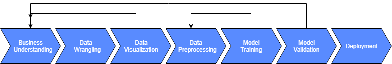
• Learning algorithms have affinity towards certain pattern of data.
• Unscaled or unstandardized data have might have unacceptable prediction
• Learning algorithms understands only number, converting text image to number is required
• Preprocessing refers to transformation before feeding to machine learning
• 学习算法对特定模式的数据具有亲和力。
• 非标準化或非标準化的数据可能具有不可接受的预测性。
• 学习算法只理解数字，需要将文字图像转换为数字，需要将文字图像转换为数字。
• 预处理指的是在送入机器学习之前的转换。
  

StandardScaler

• The StandardScaler assumes your data is normally distributed within each feature and will scale them such that the distribution is now centred around 0, with a standard deviation of 1.
• Calculate - Subtract mean of column & div by standard deviation

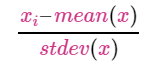
• If data is not normally distributed, this is not the best scaler to use.
• StandardScaler 假设你的数据在每个特征中是正态分布，并将对其进行缩放，使其分布以0为中心，标准差为1。
• 计算 - 减去列的平均值，然后除以标准差。
• 如果数据不是正态分布，这不是最好的缩放器。

#Generating normally distributed datadf = pd.DataFrame({'x1': np.random.normal(0, 2, 10000),'x2': np.random.normal(5, 3, 10000),'x3': np.random.normal(-5, 5, 10000)
})
df

	x1	x2	x3
0	-2.581491	7.078332	-1.098779
1	-0.618828	7.133524	-11.413612
2	3.737231	2.319060	-13.647008
3	-2.962719	6.379484	-3.626564
4	0.067544	5.490946	0.258794
...	...	...	...
9995	-4.132737	7.513709	-4.202911
9996	-1.843477	6.523104	3.327475
9997	-2.463095	3.119157	-10.941509
9998	-2.285842	-0.336564	-12.081240
9999	-2.451150	6.416026	-5.911285

10000 rows × 3 columns

# plotting data
df.plot.kde()

from sklearn.preprocessing import StandardScaler
standardscaler = StandardScaler()
data_tf = standardscaler.fit_transform(df)
#df = pd.DataFrame(data_tf, columns=['x1','x2','x3'])
df = pd.DataFrame(data_tf, columns=df.columns)
df

	x1	x2	x3
0	-1.309861	0.698005	0.770838
1	-0.329290	0.716500	-1.301191
2	1.847053	-0.896867	-1.749832
3	-1.500328	0.463815	0.263060
4	0.013630	0.166059	1.043546
...	...	...	...
9995	-2.084884	0.843904	0.147285
9996	-0.941140	0.511943	1.659978
9997	-1.250709	-0.628748	-1.206356
9998	-1.162151	-1.786789	-1.435303
9999	-1.244741	0.476061	-0.195891

10000 rows × 3 columns

df.plot.kde()

MinMaxScaler

• One of the most popular
• Calculate - Subtract min of column & div by difference between max & min

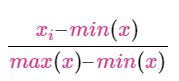
• Data shifts between 0 & 1
• If distribution not suitable for StandardScaler, this scaler works out.
• Sensitive to outliers
• 最受欢迎的产品之一
• 计算 - 减去列的最小值，再除以最大和最小值的差额。
• 数据在0和1之间移动
• 如果分布不适合于StandardScaler，这个标度器就可以工作。
• 对离群值很敏感

df = pd.DataFrame({# positive skew'x1': np.random.chisquare(8, 1000),# negative skew 'x2': np.random.beta(8, 2, 1000) * 40,# no skew'x3': np.random.normal(50, 3, 1000)
})
df

	x1	x2	x3
0	5.307743	33.180987	46.799389
1	6.226541	37.333485	54.523607
2	2.325420	23.625218	46.881535
3	3.027399	30.938227	52.743865
4	4.313804	34.570459	51.055439
...	...	...	...
995	6.405312	29.748700	50.520627
996	5.593494	37.662222	54.567921
997	15.937442	24.797026	47.477008
998	10.811419	37.077553	49.496734
999	2.120377	25.686368	53.732740

1000 rows × 3 columns

df.plot.kde()

from sklearn.preprocessing import MinMaxScaler
minmax = MinMaxScaler()
data_tf = minmax.fit_transform(df)
df = pd.DataFrame(data_tf,columns=df.columns)
df.plot.kde()

Robust Scaler|鲁棒的缩放器

• Suited for data with outliers
• Calculate by subtracting 1st-quartile & div by difference between 3rd-quartile & 1st-quartile
  
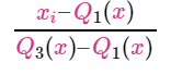
• 适用于有离群值的数据
• 减去第1个四分位数，再除以第3个四分位数和第1个四分位数之间的差额计算。

df = pd.DataFrame({# Distribution with lower outliers'x1': np.concatenate([np.random.normal(20, 1, 1000), np.random.normal(1, 1, 25)]),# Distribution with higher outliers'x2': np.concatenate([np.random.normal(30, 1, 1000), np.random.normal(50, 1, 25)]),
})

df.plot.kde()

from sklearn.preprocessing import RobustScaler
robustscaler = RobustScaler()
data_tf = robustscaler.fit_transform(df)
df = pd.DataFrame(data_tf, columns=df.columns)

df.plot.kde()

Normalizer归一化器

• Each parameter value is obtained by dividing by magnitude
  
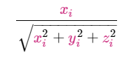
• Centralizes data to origin
• 每个参数值都是用幅度除以大小得出的。
• 将数据集中到原点

df = pd.DataFrame({'x1': np.random.randint(-100, 100, 1000).astype(float),'y1': np.random.randint(-80, 80, 1000).astype(float),'z1': np.random.randint(-150, 150, 1000).astype(float),
})

fig = plt.figure()
ax = plt.axes(projection='3d')
ax.scatter3D(df.x1, df.y1, df.z1)

from sklearn.preprocessing import Normalizer
normalizer = Normalizer()
data_tf = normalizer.fit_transform(df)
df = pd.DataFrame(data_tf, columns=df.columns)

ax = plt.axes(projection='3d')
ax.scatter3D(df.x1, df.y1, df.z1)

Binarization|二进制化

• Thresholding numerical values to binary values ( 0 or 1 )
• A few learning algorithms assume data to be in Bernoulli distribution - Bernoulli’s Naive Bayes
• 阈值为二进制值（0或1）。
• 少数学习算法假设数据处于Bernoulli分布中 - Bernoulli’s Naive Bayes

X = np.array([[ 1., -1.,  2.],[ 2.,  0.,  0.],[ 0.,  1., -1.]])

from sklearn.preprocessing import Binarizer
binarizer = Binarizer()
data_tf = binarizer.fit_transform(X)
data_tf

array([[1., 0., 1.],[1., 0., 0.],[0., 1., 0.]])

Encoding Categorical Values |编码分类值

Encoding Ordinal Values|编码顺序值

• Ordinal Values - Low, Medium & High. Relationship between values
• LabelEncoding with right mapping
• 顺序值–低、中、高。值之间的关系
• 标签编码与正确的映射

df = pd.DataFrame({'Age':[33,44,22,44,55,22],'Income':['Low','Low','High','Medium','Medium','High']})
df
df.Income=df.Income.map({'Low':1,'Medium':2,'High':3})

df

	Age	Income
0	33	1
1	44	1
2	22	3
3	44	2
4	55	2
5	22	3

PS: We can use transformer class for this as well, we will see that later|我们也可以用变压器类来做这个，我们稍后会看到。

Encoding Nominal Values|编码标称值

• Nominal Values - Male, Female. No relationship between data
• One Hot Encoding for converting data into one-hot vector
• 名义值–男性、女性。数据之间没有关系
• 独热编码，用于将数据转换为一热向量。

df = pd.DataFrame({'Age':[33,44,22,44,55,22],'Gender':['Male','Female','Male','Female','Male','Male']})
df.Gender.unique()

array(['Male', 'Female'], dtype=object)

from sklearn.preprocessing import LabelEncoder,OneHotEncoder
le = LabelEncoder()
df['gender_tf'] = le.fit_transform(df.Gender)
df

	Age	Gender	gender_tf
0	33	Male	1
1	44	Female	0
2	22	Male	1
3	44	Female	0
4	55	Male	1
5	22	Male	1

df=df.drop(['Gender'],axis=1)
df

	Age	gender_tf
0	33	1
1	44	0
2	22	1
3	44	0
4	55	1
5	22	1

OneHotEncoder().fit_transform(df[['gender_tf']]).toarray()

d:\Anaconda3\lib\site-packages\sklearn\preprocessing\_encoders.py:415: FutureWarning: The handling of integer data will change in version 0.22. Currently, the categories are determined based on the range [0, max(values)], while in the future they will be determined based on the unique values.
If you want the future behaviour and silence this warning, you can specify "categories='auto'".
In case you used a LabelEncoder before this OneHotEncoder to convert the categories to integers, then you can now use the OneHotEncoder directly.warnings.warn(msg, FutureWarning)array([[0., 1.],[1., 0.],[0., 1.],[1., 0.],[0., 1.],[0., 1.]])

Imputation|缺失值填补

• Missing values cannot be processed by learning algorithms
• Imputers can be used to infer value of missing data from existing data
• 缺失的值无法被学习算法处理。
• 可使用Imputers从现有数据中推断出缺失数据的价值。

df = pd.DataFrame({'A':[1,2,3,4,np.nan,7],'B':[3,4,1,np.nan,4,5]
})

from sklearn.preprocessing import Imputer
imputer = Imputer(strategy='mean', axis=1)

d:\Anaconda3\lib\site-packages\sklearn\utils\deprecation.py:66: DeprecationWarning: Class Imputer is deprecated; Imputer was deprecated in version 0.20 and will be removed in 0.22. Import impute.SimpleImputer from sklearn instead.warnings.warn(msg, category=DeprecationWarning)

imputer.fit_transform(df)

array([[1., 3.],[2., 4.],[3., 1.],[4., 4.],[4., 4.],[7., 5.]])

'''|  strategy : string, optional (default="mean")|      The imputation strategy.|  |      - If "mean", then replace missing values using the mean along|        the axis.|      - If "median", then replace missing values using the median along|        the axis.|      - If "most_frequent", then replace missing using the most frequent|        value along the axis.|  |  axis : integer, optional (default=0)|      The axis along which to impute.|  |      - If `axis=0`, then impute along columns.|      - If `axis=1`, then impute along rows.
'''
help(Imputer)

Polynomial Features|多项式特征

• Deriving non-linear feature by coverting data into higher degree
• Used with linear regression to learn model of higher degree
• 通过将数据隐蔽到更高的度数，推导出非线性特征。
• 与线性回归一起使用，用于学习更高的模型。

df = pd.DataFrame({'A':[1,2,3,4,5], 'B':[2,3,4,5,6]})
print(df)
from sklearn.preprocessing import PolynomialFeatures
pol = PolynomialFeatures(degree=2)
pol.fit_transform(df)

   A  B
0  1  2
1  2  3
2  3  4
3  4  5
4  5  6array([[ 1.,  1.,  2.,  1.,  2.,  4.],[ 1.,  2.,  3.,  4.,  6.,  9.],[ 1.,  3.,  4.,  9., 12., 16.],[ 1.,  4.,  5., 16., 20., 25.],[ 1.,  5.,  6., 25., 30., 36.]])

Custom Transformer |自定义变压器

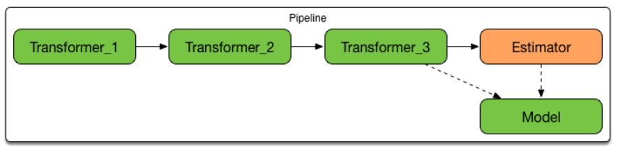
• Often, you will want to convert an existing Python function into a transformer to assist in data cleaning or processing.
• FunctionTransformer is used to create one Transformer
• validate = False, is required for string columns
• 通常情况下，你会想把一个现有的Python函数转换为一个变换器来协助数据清理或处理。
• FunctionTransformer用于创建一个Transformer。
• validate = False，对于字符串列来说是必须的。

from sklearn.preprocessing import FunctionTransformerdef mapping(x):x['Age'] = x['Age']+2x['Counter'] = x['Counter'] * 2return xcustomtransformer = FunctionTransformer(mapping, validate=False)

df = pd.DataFrame({'Age':[33,44,22,44,55,22],'Counter':[3,4,2,4,5,2],})
print(df)
customtransformer.transform(df)

   Age  Counter
0   33        3
1   44        4
2   22        2
3   44        4
4   55        5
5   22        2

	Age	Counter
0	35	6
1	46	8
2	24	4
3	46	8
4	57	10
5	24	4

Text Processing|文本处理

• Perhaps one of the most common information
• Learning algorithms don’t understand text but only numbers
• Below menthods convert text to numbers

CountVectorizer

• Each column represents one word, count refers to frequency of the word
• Sequence of words are not maintained

Hyperparameters|超参数

• n_grams - Number of words considered for each column

• stop_words - words not considered

• vocabulary - only words considered

• 也许是最常见的信息之一

• 学习算法不理解文本，只理解数字。

• 以下方法将文字转换为数字

• 每栏代表一个单词，计数是指单词的频率。

• 没有保持字的顺序

• n_grams - 每栏考虑的字数

• stop_words - 不考虑的单词

• 词汇量 – -- 只考虑词汇

corpus = ['This is the first document awesome food.','This is the second second document.','And the third one the is mission impossible.','Is this the first document?',
]
df = pd.DataFrame({'Text':corpus})
df

	Text
0	This is the first document awesome food.
1	This is the second second document.
2	And the third one the is mission impossible.
3	Is this the first document?

from sklearn.feature_extraction.text import CountVectorizer
cv = CountVectorizer()
cv.fit_transform(df.Text).toarray()

array([[0, 1, 1, 1, 1, 0, 1, 0, 0, 0, 1, 0, 1],[0, 0, 1, 0, 0, 0, 1, 0, 0, 2, 1, 0, 1],[1, 0, 0, 0, 0, 1, 1, 1, 1, 0, 2, 1, 0],[0, 0, 1, 1, 0, 0, 1, 0, 0, 0, 1, 0, 1]], dtype=int64)

cv.vocabulary_

{'this': 12,'is': 6,'the': 10,'first': 3,'document': 2,'awesome': 1,'food': 4,'second': 9,'and': 0,'third': 11,'one': 8,'mission': 7,'impossible': 5}

cv = CountVectorizer(stop_words=['the','is'])
cv.fit_transform(df.Text).toarray()

array([[0, 1, 1, 1, 1, 0, 0, 0, 0, 0, 1],[0, 0, 1, 0, 0, 0, 0, 0, 2, 0, 1],[1, 0, 0, 0, 0, 1, 1, 1, 0, 1, 0],[0, 0, 1, 1, 0, 0, 0, 0, 0, 0, 1]], dtype=int64)

cv.vocabulary_

{'this': 10,'first': 3,'document': 2,'awesome': 1,'food': 4,'second': 8,'and': 0,'third': 9,'one': 7,'mission': 6,'impossible': 5}

cv = CountVectorizer(vocabulary=['mission','food','second'])
cv.fit_transform(df.Text).toarray()

array([[0, 1, 0],[0, 0, 2],[1, 0, 0],[0, 0, 0]], dtype=int64)

cv = CountVectorizer(ngram_range=[1,2])
cv.fit_transform(df.Text).toarray()

array([[0, 0, 1, 1, 1, 1, 1, 1, 1, 0, 1, 0, 1, 0, 0, 0, 0, 0, 0, 0, 0, 1,1, 0, 0, 0, 0, 0, 1, 1, 0],[0, 0, 0, 0, 1, 0, 0, 0, 0, 0, 1, 0, 1, 0, 0, 0, 0, 0, 2, 1, 1, 1,0, 0, 1, 0, 0, 0, 1, 1, 0],[1, 1, 0, 0, 0, 0, 0, 0, 0, 1, 1, 1, 0, 0, 1, 1, 1, 1, 0, 0, 0, 2,0, 1, 0, 1, 1, 1, 0, 0, 0],[0, 0, 0, 0, 1, 0, 1, 1, 0, 0, 1, 0, 0, 1, 0, 0, 0, 0, 0, 0, 0, 1,1, 0, 0, 0, 0, 0, 1, 0, 1]], dtype=int64)

cv.vocabulary_

{'this': 28,'is': 10,'the': 21,'first': 6,'document': 4,'awesome': 2,'food': 8,'this is': 29,'is the': 12,'the first': 22,'first document': 7,'document awesome': 5,'awesome food': 3,'second': 18,'the second': 24,'second second': 20,'second document': 19,'and': 0,'third': 26,'one': 16,'mission': 14,'impossible': 9,'and the': 1,'the third': 25,'third one': 27,'one the': 17,'the is': 23,'is mission': 11,'mission impossible': 15,'is this': 13,'this the': 30}

TfIdfVectorizer

• Words occuring more frequently in a doc versus entire corpus is considered more important
• The importance is in scale of 0 & 1
• 词组中出现频率较高的词组被认为更重要。
• 重要程度以0和1为单位。

from sklearn.feature_extraction.text import TfidfVectorizer
vectorizer = TfidfVectorizer(stop_words='english')

vectorizer.fit_transform(df.Text).toarray()

array([[0.64450299, 0.41137791, 0.64450299, 0.        , 0.        ,0.        ],[0.        , 0.30403549, 0.        , 0.        , 0.        ,0.9526607 ],[0.        , 0.        , 0.        , 0.70710678, 0.70710678,0.        ],[0.        , 1.        , 0.        , 0.        , 0.        ,0.        ]])

vectorizer.get_feature_names()

['awesome', 'document', 'food', 'impossible', 'mission', 'second']

HashingVectorizer

• All above techniques converts data into table where each word is converted to column
• Learning on data with lakhs of columns is difficult to process
• HashingVectorizer is an useful technique for out-of-core learning
• Multiple words are hashed to limited column
• Limitation - Hashed value to word mapping is not possible
• 以上所有技术都将数据转换为表格，其中每个字都被转换为列。
• 在有几百万列的数据上学习很难处理
• HashingVectorizer是一种有用的核心外学习技术。
• 多个单词被散列到有限的列中
• 限制----不可能对单词进行哈希值映射。

from sklearn.feature_extraction.text import HashingVectorizer
hv = HashingVectorizer(n_features=5)

hv.fit_transform(df.Text).toarray()

array([[ 0.        , -0.37796447,  0.75592895, -0.37796447,  0.37796447],[ 0.81649658,  0.        ,  0.40824829, -0.40824829,  0.        ],[-0.31622777,  0.        ,  0.31622777, -0.63245553, -0.63245553],[ 0.        , -0.57735027,  0.57735027, -0.57735027,  0.        ]])

Image Processing using skimage|使用skimage进行图像处理

• skimage doesn’t come with anaconda. install with ‘pip install skimage’
• Images should be converted from 0-255 scale to 0-1 scale.
• skimage takes image path & returns numpy array
• images consist of 3 dimension
• skimage不附带anaconda，用’pip install skimage’安装。
• 图像应从0-255比例转换为0-1比例。
• skimage取图像路径并返回numpy数组。
• 图像由3个维度组成

from skimage.io import imread,imshow
image = imread('Data\cat.jpg')

image.shape

(539, 461, 3)

image[0]

Array([[164, 157, 151],[164, 157, 151],[164, 157, 151],...,[199, 195, 192],[199, 195, 192],[199, 195, 192]], dtype=uint8)

imshow(image)

from skimage.color import rgb2gray

rgb2gray(image).shape

(539, 461)

imshow(rgb2gray(image))

from skimage.transform import resize

imshow(resize(image, (200,200)))

使用scikit-learn进行预处理相关推荐

1. 机器学习与Scikit Learn学习库

   摘要: 本文介绍机器学习相关的学习库Scikit Learn,包含其安装及具体识别手写体数字案例,适合机器学习初学者入门Scikit Learn. 在我科研的时候,机器学习(ML)是计算机科学领域中最 ...

2. Scikit Learn: 在python中机器学习

   Warning 警告:有些没能理解的句子,我以自己的理解意译. 翻译自:Scikit Learn:Machine Learning in Python 作者: Fabian Pedregosa, Ga ...

3. [转载]Scikit Learn: 在python中机器学习

   原址:http://my.oschina.net/u/175377/blog/84420 目录[-] Scikit Learn: 在python中机器学习 载入示例数据 一个改变数据集大小的示例:数码 ...

4. 【scikit-learn】如何用Python和SciKit Learn 0.18实现神经网络

   本教程的代码和数据来自于 Springboard 的博客教程.本文的作者为 Jose Portilla,他是网络教育平台 Udemy 一门数据科学类课程的讲师. GitHub 链接:https://g ...

5. scikit - learn 做文本分类

   文章来源: https://my.oschina.net/u/175377/blog/84420 Scikit Learn: 在python中机器学习 Warning 警告:有些没能理解的句子,我以自 ...

6. python笔迹识别_python_基于Scikit learn库中KNN,SVM算法的笔迹识别

   之前我们用自己写KNN算法[网址]识别了MNIST手写识别数据 [数据下载地址] 这里介绍,如何运用Scikit learn库中的KNN,SVM算法进行笔迹识别. 数据说明: 数据共有785列,第一列 ...

7. python scikit learn 关闭开源_scikit learn 里没有神经网络？

   本教程的代码和数据来自于 Springboard 的博客教程,希望能为你提供帮助.作者为 Jose Portilla,他是网络教育平台 Udemy 一门数据科学类课程的讲师. GitHub 链接:ht ...

8. python 高维数据_用Sci-kit learn和XGBoost进行多类分类：Brainwave数据案例研究

   在机器学习中,高维数据的分类问题非常具有挑战性.有时候,非常简单的问题会因为这个"维度诅咒"问题变得非常复杂.在本文中,我们将了解不同分类器的准确性和性能是如何变化的. 理解数据 ...

9. python scikit learn 关闭开源_慕课|Python调用scikit-learn实现机器学习(一）

   一.机器学习介绍及其原理 1.什么是人工智能? 机器对人的思维信息过程的模拟,让它能相认一样思考. a.输入 b.处理 c.输出 根据输入信息进行模型建构.权重更新,实现最终优化. 特点:信息处理.自 ...

10. python基于svm的异常检测_[scikit learn]：异常检测-OneClassSVM的替代方案

    不幸的是,scikit目前只学习implements一类支持向量机和用于离群点检测的鲁棒协方差估计 通过检查2d数据上的差异,可以尝试比较这些方法(as provided in the doc):im ...

最新文章

1. Vue 系列之 组件
2. 你应该掌握的七种回归技术
3. netbeans工具栏字体太小
4. java 死锁的检测与修复_调查死锁–第4部分：修复代码
5. nginx下gzip配置参数详解
6. 和项目组研究计算几何
7. 为什么无法建立过程性能模型？
8. 深入浅出Python机器学习3——K最近邻算法
9. DS1302时钟模块简单介绍
10. 前端进阶之——CSS背景、字体和文本样式
11. 学习笔记Android弹框material-dialogs
12. 雷尼绍Renishaw wdf 文件解析(Python源码)软件分享
13. win2008计算机无法访问,win2008共享资源无法访问故障的应对措施
14. 基于MATLAB分析,基于Matlab对信号进行频域分析的方法
15. vue的三种传值方式：父传子，子传父，子传子
16. office 所有后缀对应的 content-type
17. C语言给小学生出题（随机1~99进行四则运算）
18. devops包括什么_名字叫什么？ DevOps版。
19. 盈一眸恬淡，在明媚的春天等你
20. Pandas 基础知识

热门文章

1. 一个用户实体应该有它自己的实体验证,即一个实体应该有它的属性,方法,扩展属性及验证机制组成...
2. SQL Server 2016 查询存储性能优化小结
3. 德国蓝皮书：解决特定问题 德国渐进建设智慧城市
4. Memcached全面剖析
5. NodeJs教程(介绍总结！)终于在网上找到一个靠谱点的了T_T
6. tcp wrapper
7. 符合标准的TreeView实现(Div+CSS+JS+ASP.NET)
8. Ubuntu16.04中WPS不能输入中文
9. php sapi linux,PHP内核 - SAPI - Cli
10. 打开网页时出现DA AddrBar icon的解决方法